KESA – Event Sourcing
KESA - Event Sourcing Illustrated: A Jigsaw Puzzle Game Perspective
In the dynamic world of software development, managing and maintaining the state of an application poses significant challenges. Event sourcing, an innovative architectural pattern, steps in to revolutionize this process, which offers a robust foundation for understanding not only where the system stands, but also how it got there, significantly enhancing both transparency and traceability.
What is Event Sourcing?
Event sourcing is an architectural pattern that captures changes to an entity's state through a chronological series of events. This approach diverges from traditional methodologies that emphasize storing the current state, by instead focusing on the sequence of events that lead to that state.
Event Sourcing utilizes concepts such as events, event streams, event stores, and event handlers to manage and process these changes. Further, it offers benefits such as immutable event logs, auditability, event replay for state reconstruction, consistency, improved scalability, fault tolerance, and support for event-driven architectures.
Jigsaw Puzzle Game Project Overview
To illustrate the practical application of event sourcing, we present a simple, engaging example: a digital jigsaw puzzle game. This single-player game is developed to highlight the principles and advantages of event sourcing and event-driven architectures, where a player interacts with a web interface to assemble a jigsaw puzzle.
Play the game here: Fidenz Kesa
Find instructions on how to play here
Find the full project explainer video here: https://youtu.be/4O9VukIrtCI
Implementing Event Sourcing in Jigsaw Puzzle Game
The table below demonstrates the implementation of event sourcing features within the Jigsaw Puzzle Game application, which has been intentionally over-engineered to effectively illustrate event sourcing capabilities using a jigsaw puzzle game as an example.
| Event Sourcing Feature | Application Implementation | Benefits in the Game Context |
|---|---|---|
| Entity | The "JigsawPuzzleGame" entity is designed to represent the current state of a gaming session. | Encapsulates the game logic and helps validating events for an ongoing gaming session |
| Event | Each game action triggering an event sent from the front-end to the back-end such as: Game Started Event, Piece Added Event, Piece Removed Event. | Facilitates real-time game interactions and state management |
| Event Stream | A gaming session begins with a Start Game Event, marking the commencement of an event stream. Subsequent events, including Piece Added Events and Piece Removed Events, will be sequentially numbered in chronological order. | Ensures ordered, reliable processing of game actions |
| Event Handlers | Event handlers are designed to react to various events, taking actions such as processing data and updating “JigsawPuzzleGame” entity. | Enables dynamic game state management based on player actions |
| Event Store | Events are stored in the event store and can be retrieved as needed. Once saved, these events are immutable. Each event record includes essential information such as the unique game session ID, event type, event stream ID, and event data, among other details. | Provides durability and historical tracking of game actions |
| Immutable Event Log | Event Store implementation provide chronologically ordered immutable events of a gaming session | Accurate tracking of puzzle progress |
| Event Replay | A Player can use the Event List to go back in time to a specific point in the game. This can be done by selecting an event from the event list. The system then reverse all subsequent events by applying their opposite, thus restoring the puzzle to the desired state |
Ability to revert puzzle state and understand puzzle assembly |
| Consistency and Eventual Consistency | Storing events in chronological order with event stream ID and event type | Distinguishes between the various events that occur within a gaming session. |
Conclusion
The jigsaw puzzle game serves as a practical and engaging example to illustrate the principles of event sourcing. By understanding how each action in the game translates into an event and contributes to the puzzle's state, we can appreciate the power and utility of event sourcing in software development. As technology evolves, it's exciting to ponder how event sourcing will shape the future of data management and application design.
Instructions and How to play this game
- Watch the video below for instructions on how to play the game.
- Interact with a dual-panel interface: left panel for puzzle assembly, right panel for displaying available jigsaw pieces.
- First, choose a puzzle size from three game size options: 4x4, 5x5 (default), or 6x6.
- Start the game using start button
- Upon start four puzzle pieces will be available in the piece viewer for selection.
- Add pieces by dragging them from the piece viewer to the grid.
- Remove pieces by clicking on a piece in the grid and confirming the subsequent pop-up.
- Removed pieces won't be added back to the piece viewer but will be available for future selection.
- Use the “Re-shuffle” button to refresh the piece selection with a new set of random pieces, useful when the piece viewer is empty.
- Reset the game at any time using the “Reset” button.
- Event List Panel
- To view the events occurred while playing the game
- To Revert puzzle to a previous state by selecting an event in the event list and confirming the prompted pop-up.
The game concludes when the puzzle is fully assembled, with completion time affecting the player's score.
Would you like to learn more? Contact Us!
If you have any additional questions about this or would like a word with our creators? Feel free to reach out to us.
📆 Talk to Us: Contact us - Fidenz Technologies
Keep an eye out for our upcoming content from Fidenz Technologies, as we embark on a journey through the intricate realms of technology.
Happy Exploring!
Why Kubernetes On-Prem and a Glimpse into Our Setup
Introduction
Deploying a Kubernetes on-prem cluster may pose challenges, but it grants complete control over hardware, allowing customization of infrastructure to specific needs. Data is stored securely within our organization's premises, eliminating recurring costs for the same resources. Additionally, the setup allows for performance optimization and avoids network overhead.
let's see why we would need a Kubernetes on prem cluster.
Why Kubernetes On-Prem?
Embarking on the deployment of a Kubernetes cluster on-premises is undeniably accompanied by inherent challenges; however, there exist compelling scenarios that necessitate this strategic decision. The stringent demands of regulatory compliance, coupled with heightened security considerations, often drive organizations towards on-premises deployment. Furthermore, the seamless integration with pre-existing infrastructure and the pursuit of optimized performance, especially in scenarios requiring low-latency workloads, reinforce the appeal of on-premises Kubernetes deployment. In the intricate landscape of modern IT, these considerations collectively underscore the relevance of on-premises solutions despite their inherent complexities.
How we deployed our own Kubernetes on-Prem cluster
When considering the deployment of a Kubernetes on-premises cluster, it's essential to take into account factors such as the storage provisioner, load balancing, cluster autoscaling, and high availability. We opted for a canonical stack to facilitate the deployment of our on-premises cluster, aiming to achieve automated cluster deployment and configure high availability seamlessly.
We leveraged MAAS (Metal as a Service) for infrastructure provisioning. MAAS is a robust tool that streamlines the deployment of physical servers, allowing for efficient management and provisioning in a data center or on-premises environment.
To orchestrate the cluster deployment, we employed Juju. Juju is a powerful application modeling tool that simplifies the management and scaling of complex software infrastructure. It facilitates the seamless deployment and integration of applications across various cloud and on-premises environments.
Now, let's delve into the steps and measures we undertook to successfully deploy our own Kubernetes on-premises cluster
Features provided by our on-premise Kubernetes cluster
- Persistent Storage
- We chose Ceph as our storage provisioner, leveraging Juju for both the deployment and configuration of the Ceph cluster. With features like storage pooling and replication, Ceph ensures a highly available storage provisioner, meeting our requirements for resilience and redundancy in the storage infrastructure.
- High Availability
- With Juju, we could deploy multiple control nodes, ensuring easy availability, and set up multiple etcd and Ceph servers for enhanced resilience and availability. This approach enhances the reliability of our infrastructure by distributing critical components across redundant nodes, minimizing the risk of single points of failure.
- Cluster Autoscaling
- Utilizing the Charmed Kubernetes Autoscaler, we've automated node autoscaling within our Kubernetes cluster, dynamically adding or removing worker nodes as needed. This not only ensures optimal resource utilization but also contributes to cost efficiency by automatically adjusting the cluster size based on workload demands. The autoscaler is a valuable tool for maintaining an agile and resource-efficient on-premises Kubernetes environment.
- Load Balancing
- With the integration of MetalLB as our load balancer, we enhance the scalability and distribution of network traffic within the cluster. MetalLB is a versatile load balancing solution designed for bare-metal Kubernetes deployments. It dynamically assigns external IP addresses to services, allowing for efficient load balancing and seamless traffic management across the Kubernetes nodes in our on-premises cluster.
Feel free to refer to our second article for a more in-depth exploration of why we opt for Kubernetes on-premises and a detailed comparison highlighting the distinctions between on-premises and cloud deployments.
Now, please head down to our video to delve a bit deeper into these topics and take a closer look at our deployed Kubernetes on-premises cluster.
📽️ Watch Video: Why Kubernetes On-Prem and a Glimpse into Our Setup
Would you like to learn more? Contact Us!
If you have any additional questions about this or require a similar service, feel free to reach out to us. We're here to assist you and explore how we can meet your specific needs.
📆 Talk to Us: Talk to Creators
Keep an eye out for our upcoming content from Fidenz Technologies, as we embark on a journey through the intricate realms of technology. Join us for in-depth explorations, insightful discussions, and a continuous stream of technological adventures that promise to expand your knowledge and keep you informed about the latest trends and developments in the ever-evolving tech landscape.
Until then, happy exploring!
KEDAS: SYNC RELATIONAL AND NON-RELATIONAL DATABASES USING KAFKA
Background
In the era of digitalization, the landscape of data has evolved dramatically. Initially used for monitoring and analysis, data quickly became a vital asset for real-time decision-making. As data volumes soared, the value of static information dwindled, while the significance of continuous data streams skyrocketed. Within this dynamic context, Kafka emerged as a pivotal tool for data management.
What is Kafka?
Kafka lies at the heart of this data revolution as an event streaming platform. It excels at capturing data from diverse sources, seamlessly processing, storing, and delivering it to those who seek actionable insights. While Kafka shares similarities with traditional pub-sub message queues like RabbitMQ, it sets itself apart in several critical ways:
- Operates as a modern distributed system
- Offers robust data storage capabilities
- Processes data streams, creating new events beyond traditional message brokering
Purpose of this Project
Recognizing Kafka's versatility and surging popularity, we embarked on a journey to harness its capabilities for delivering superior solutions to our clients.
Our mission? To dive deep into this technology and build an innovative solution leveraging Kafka’s capability.
Project Overview
KEDAS is a data synchronization application designed to work seamlessly across various database servers, including MS SQL, MySQL, PostgreSQL, and more. In an effort to enhance versatility and complexity, we extended its capabilities to facilitate synchronization between both relational and non-relational databases. Unlike most data synchronization tools available, our solution allows changes made in one data source to be seamlessly synchronized with multiple data sources through minimum configurations.
This project stands as a testament to our commitment to embracing innovative technologies like Kafka to offer cutting-edge solutions to our clients. As data continues to be a driving force in the digital landscape, Kafka remains at the forefront of efficient and real-time data management, enabling us to deliver exceptional results.
Outcomes
We have developed a Kafka processor and a set of Kafka connectors to enable data synchronization between different data sources. To make the system testable, we have developed a simple web application that interacts with two independent databases which are synchronized using our KEDAS.
Kafka Demo App
Check out the video below to get a quick overview of how everything works together and if you like to try how this works, try it yourself with our demo application.
Demo Video: Kedas Demo
Try it yourself: Kedas Dashboard
Want to know more about Kafka based solutions? Talk to Creators
For more information and updates on Kafka-driven projects by Fidenz, stay tuned. Follow us for the latest updates!
A CNN Approach for Recognizing Traffic Signs
Introduction
Deep Learning is an interesting and a unique field of study that has attracted the worldwide attention over the past few years at a rapid pace. The rate at which the digitalized systems have been generating data for over a decade, has become one of the major reasons for creating an abundance of data. As a result, the availability of data provided a brand new perspective for the researchers to look at Artificial Intelligence and its branches, in a different way. Additionally, the gradual enhancement of hardware resources resulted in offering much improved computational resources for the deep learning researchers to make use of data efficiently. Therefore, the combination of data and modern computational resources, was able to create a platform for the researchers to thrive on, and the result is a highly motivated deep learning community that continues to contribute towards the growth of deep learning using novel approaches. Computer vision is a research area that has benefitted largely from the rise of deep learning, and it is evident from the amount of research studies carried out in computer vision with deep learning.
While there are many specific applications of computer vision, the uses of deep learning in traffic/road related applications, is an interesting application since it directly affects the improvement of vehicular automation. Although the field of vehicular automation is on the verge of reaching greater heights, as evident from Tesla’s Autopilot feature (and similar implementations from other major automobile manufacturers), understanding the fundamentals of deep learning remains an integral part for those who are interested in exploring the capabilities of deep learning. In this article, we focus on bringing you a primer for understanding how the nuts and bolts of deep learning can effectively improve the metrics that measure the success of a specific application that targets traffic signs. Thus, our attempt is to explore the process of developing a traffic sign recognizer using the concepts of deep learning.
We have structured the article in way that allows you to easily move to the desired section with ease. Initially, we explain the Background behind the problem before coming up with an Exploratory Data Analysis for the dataset which we utilized. Afterwards, the Deep Learning Workflow provides a high-level overview of the procedure followed by us, and then we place our emphasis on creating a suitable Input Pipeline for preparing the data to meet the requirements of the Models explained in the subsequent section. Finally, we examine the performance of the developed model, before capping the article off by deploying it as a readymade model which can be tested by yourself using an interactive interface. Sounds interesting, huh?
Background
The Problem
A brief writeup on the actual problem that we are attempting to address. In our context, the broader problem is to check the possibility of recognizing the traffic signs via the concepts of computer vision.
What will straightly come to your mind if you are asked to think of a main road in any part of the world? Obviously, the pedestrians and vehicles should greet your mind as they make the roads busy, thanks to the continuous movements made by them. The clutters of vehicles and pedestrians can certainly lead to unpleasant outcomes, and as a result, standardized road rules have been set up by the authorities to minimize the clutters and to streamline the traffics in a structured manner. Since the drivers and pedestrians are supposed to obey the rules, having assistive signs/lights can definitely help both the drivers and pedestrians to ensure that the road is a safe environment for everyone.
This is where the importance of traffic signs, comes into the frame to act as guidelines for both drivers and pedestrians. While the traffic signs are supposed to be understood by human vision, it is interesting to if the same phenomenon can be emulated using computer vision. In this article, we attempt to address a basic problem, in which we check the possibility of recognizing the traffic signs via the concepts of computer vision.
The Aim (and objectives)
In a broader context, our aim is to develop a recognizer that correctly classifies a given traffic sign image to determine its class, using the concepts of deep learning in computer vision. It is expected to achieve the aim by methodically following the objectives given below.
- Exploring the health of the dataset by performing an Exploratory Data Analysis
- Preprocessing the data for building the input pipeline
- Defining a suitable methodology that iteratively improves the performance of the model.
- Testing the performances on unseen datasets.
- Developing a tool for allowing the user to self-test the capabilities of the developed model.
The Dataset
As we explained in the Introduction section, datasets play a pivotal role in the development of a deep learning based solution. Fortunately, there are freely available datasets for achieving our requirement. Therefore, we used the German Traffic Sign Recognition Benchmark (GTSRB) dataset provided by the Institut für Neuroinformatik. The dataset has been initially provided as a multi-class classification challenge at the International Joint Conference on Neural Networks (IJCNN) 2011.
Exploratory Data Analysis
The Exploratory Data Analysis (EDA) is a common component that provides a representation of the original dataset using descriptive statistical methods with the aid of relevant plots. For more information, refer the following link:
What is Exploratory Data Analysis?
Once we downloaded the ZIP file from the source given above, we came across datasets corresponding to three distinct categories inside the ZIP archive: Train, Test, and Meta. The images related to the Train dataset were stored inside the Train folder where separate sub-folders had been created to organize the Train images under different class labels. In contrast, the images related to the Test dataset were directly inside a folder named Test. The Meta folder was composed of computer-illustrated images to represent each class label and few of the images from all three categories are given below. Additionally, the archive contained three annotated Comma Separated Files (CSV) named Train.csv, Test.csv, and Meta.csv. The composition of each CSV file, is further discussed within this section in the following paragraphs.
Train
Sample Image from the Dataset

Number of Images
In order to explore the number of available images in the Train dataset, the Train.csv file can be analyzed. The Pandas library in Python is a useful tool for dealing with CSV files by including the data into a Dataframe. Based on the results, the dataset contained 39,209 images.
Number of Classes
The dataset consists of images corresponding to 43 classes, numbered sequentially from 0 to 42.
Class Distribution
The following figure represents the class distribution of the Train dataset.

Structure of Data
Altogether, the Train.csv file contains the following list of important fields which can be utilized as per the requirements [Ref: German Traffic Sign Benchmarks ]
- Width: The width of the image in pixels
- Height: The width of the image in pixels
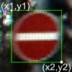
- Roi.X1: The X-coordinate of top-left corner of traffic sign bounding box
- Roi.Y1: The Y-coordinate of top-left corner of traffic sign bounding box
- Roi.X2: The X-coordinate of bottom-right corner of traffic sign bounding box
- Roi.Y2: The Y-coordinate of bottom-right corner of traffic sign bounding box
- ClassId: The actual class label
Test
The annotated file for the Test dataset (Test.csv) also follows a layout similar to the Train.csv.
Sample Images from the Dataset

Number of Images
The Test dataset consists of 12,630 images as per the actual images in the Test folder and as per the annotated Test.csv file.
Number of Classes
As expected, The Test dataset also consists of images corresponding to 43 classes, numbered sequentially from 0 to 42.
Class Distribution
The following figure represents the class distribution of the Test dataset.

Meta

The Meta Dataset, along with the Meta.csv has been provided as a guideline to represent the actual images and the related Class labels.
The Deep Learning Workflow
Here, we will add a high level diagram for explaining the iterative workflow that we follow throughout the model development/improvement process. The diagram will represent the usual Machine/Deep Learning workflow, with specific customizations to cater the expected outcomes of our case study.
Over the years, the machine learning community has adopted a certain workflow that keeps them in the hunt for the reaching the desired aims and objectives. The following figure depicts the workflow which we usually follow in the process of developing machine/deep learning applications. In reality, deep learning is a highly iterative process that requires the developers to keep experimenting until the target objectives are achieved.
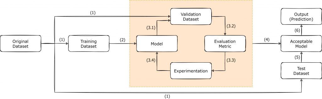
As shown in the above figure, once we have a dataset which is suitable to be applied for a deep learning task, the dataset is usually split into three subsets, known as Training Dataset, Validation Dataset and Test Dataset. The splitting process may vary, depending on the original dataset that you have, and in the context of GTSRB dataset, the authors had provided both the Training Dataset and Test Dataset separately. Since the Validation Dataset is not available in GTSRB dataset, it is up to the developers to decide the best possible way forward for creating a Validation dataset, depending on the application.
Once the Train/Validation/Test split is finalized, the Training Dataset is utilized for training the initial model, as shown in Step (2). The creation of the model initiates the iterative cycle where the model is tested against the Validation dataset to obtain the necessary evaluation metric. Based on the result of the evaluation metric, the developers are supposed to keep on experimenting and form a new model and follow the same cycle, until a model with a viable evaluation metric result is obtained. After the finalization of a model, it is considered as the Acceptable Model [Step (4)]. The Test Dataset consists of real-world data that the model has not previously seen and it provides us the opportunity to Test the created model against real-world data to actually see how it would eventually perform on the production run.
The Input Pipeline
In this section, the focus will be placed on the explaining the preprocessing steps which we followed, before the development of models.
For instance, the process of preparing Train/Validation/Test/StreetViewTest datasets, is explained, along with the other normalization steps taken during the process
In this section, we focus on the preparation of our original datasets according to a standard formats used in the process of practicing deep learning. Therefore, the preparation of the input pipeline can be illustrated in two separate steps where the first step is to prepare Training, Validation and Test datasets from the originally available data. Subsequently, we dive into the additional task of normalizing the inputs before sending them through the training cycle.
Initialization
Since this is the beginning of the code, first of all, it is required to import the necessary libraries which are required throughout the implementation.
import numpy as np
import pandas as pd
import matplotlib.pyplot as plt
import cv2
import tensorflow as tf
from PIL import Image
import keras
import os
from sklearn.model_selection import train_test_split
from tensorflow.python.keras import regularizers
Usually, when we deal with images, we deal with the array representations of the respective images, rather than working with the usually known JPEG or PNG (or any other image format) formats. The following code snippet shows how we load and convert the images to arrays from the originally available Train and Test image datasets. In the conversion job, we also place emphasis on making all the observations have the same shape when it comes to the representation of resolution of each observation. Therefore, each image is resized to have a resolution of 30x30 before being converted to a numpy array.
# Loading the Train Dataset
train_data = []
train_labels = []
basedir = "../Datasets/gtsrb"
classes = 43

for i in range(classes):
    path = os.path.join(basedir,'train',str(i))
    images = os.listdir(path)

    for j in images:
        print("Class: " + str(i) + " - Image: " + str(j))
        image = Image.open(path + '\\'+ j)
        image = image.resize((30,30))
        image = np.array(image)
        train_data.append(image)
        train_labels.append(i)

train_data = np.array(train_data)
train_labels = np.array(train_labels)

# Loading the Test Dataset

image_paths = []
test_data=[]
test_file_path = os.path.join(basedir, 'Test.csv')

Y_test_df = pd.read_csv(test_file_path)
Y_test_orig = Y_test_df["ClassId"].values

for short_path in Y_test_df["Path"]:
    image_paths.append(os.path.join(basedir, short_path))

for img in image_paths:
    print("Path: " + str(img))
    image = Image.open(img)
    image = image.resize((30,30))
    test_data.append(np.array(image))

X_test_orig = np.array(test_data)
In order to be used later for evaluation purposes, we created a custom traffic sign dataset from the images captured from Google Street View as well. The following code snippet shows how we imported them by following a similar approach shown in the previous code snippets.
# Loading the Custom Street View Dataset
sv_test_image_paths = []
sv_test_data=[]
sv_test_file_path = os.path.join(basedir, 'StreetView.csv')

Y_sv_test_df = pd.read_csv(sv_test_file_path)
Y_sv_test_orig = Y_sv_test_df["ClassId"].values

for short_path in Y_sv_test_df["Path"]:
    sv_test_image_paths.append(os.path.join(basedir, short_path))

for img in sv_test_image_paths:
    print("Path: " + str(img))
    image = Image.open(img).convert('RGB')
    image = image.resize((30,30))
    sv_test_data.append(np.array(image))

X_sv_test_orig = np.array(sv_test_data)
Train/Validation/Test Datasets
Since the original dataset comes with two main datasets (Train and Test), it was up to us to prepare the Validation dataset from the available data. Therefore, it was decided to keep aside a portion of the Train dataset for Validation dataset, and as a result, 20% of the Train dataset was allocated for the Validation dataset. Alternatively, you may use k-fold Cross Validation instead of the approach followed by us here in this section. The parameter {{random_state}} controls how the shuffling is applied before the splitting process. Using the same value for random_state will ensure that the results of the split datasets are reproducible on future instances.
X_train_orig, X_val_orig, Y_train_orig, Y_val_orig = train_test_split(train_data, train_labels, test_size=0.2, random_state=68)
Usually, it is very important to keep track of the shapes of the dataset arrays used throughout the implementation. The code snippet given below, displays the shapes of numpy arrays, after the splitting process. The code snippet further shows the number of training examples in the Training and Validation datasets after the split.
print ("Number of Training Examples = " + str(X_train_orig.shape[0])) // 31367
print ("Number of Validation Examples = " + str(X_val_orig.shape[0])) // 7842
print("X_train_orig shape: " + str(X_train_orig.shape))               // (31367, 30, 30, 3)
print("Y_train_orig shape: " + str(Y_train_orig.shape))               // (31367,)
print("X_val_orig shape: " + str(X_val_orig.shape))                   // (7842, 30, 30, 3)
print("Y_val_orig shape: " + str(Y_val_orig.shape))                   // (7842,)
print("X_test_orig shape: " + str(X_test_orig.shape))                 // (12630, 30, 30, 3)
print("Y_test_orig shape: " + str(Y_test_orig.shape))                 // (12630,)
print("X_sv_test_orig shape: " + str(X_sv_test_orig.shape))           // (32, 30, 30, 3)
print("Y_sv_test_orig shape: " + str(Y_sv_test_orig.shape))           // (32,)
Normalizing Inputs
Normalizing is a common practice in deep learning as it helps in speeding up the training process considerably. The normalization process is applied to all the datasets, and in this case-study, we apply a very simple normalization approach where the intensity values from each pixel, are divided by 255. The value 255 is chosen as the divider because 255 is the maximum possible intensity value.
Normalize image vectors
# Normalize image vectors
X_train = X_train_orig/255
X_val = X_val_orig/255
X_test = X_test_orig/255
X_sv_test = X_sv_test_orig/255
One-Hot Encoding
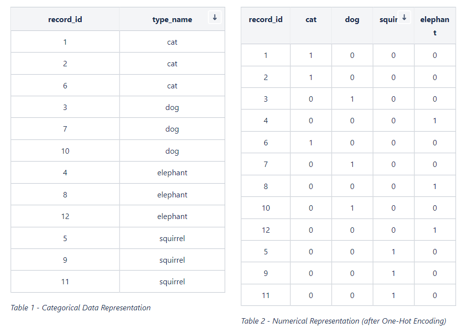
In the datasets that we are currently dealing with, we have a categorical variable as the output (i.e. 43 classes for representing the output). While some algorithms are capable of dealing with categorical data, many of the algorithms are comfortable on dealing with numerical data instead of the categorical data. One-Hot Encoding is a conversion process for representing categorical data numerically. Imagine that we are developing an animal classifier and suppose that we have cat, dog, squirrel, and elephant as the set of types of animals (as shown in Table 1). Once the One-Hot Encoding is applied to the data given in Table 1, the output becomes a numerical representation as depicted in Table 2.
For One-Hot Encoding, we use the function given below.
def convert_to_one_hot(Y, C):
    Y = np.eye(C)[Y.reshape(-1)].T
    return Y
The following code snippet shows how we applied the One-Hot Encoding to data corresponding to the output (Y) from all the available datasets. The code snippet further shows shapes of the numpy arrays after all the previously followed steps.
Y_train = convert_to_one_hot(Y_train_orig, 43).T
Y_val = convert_to_one_hot(Y_val_orig, 43).T
Y_test = convert_to_one_hot(Y_test_orig, 43).T
Y_sv_test = convert_to_one_hot(Y_sv_test_orig, 43).T

print ("Number of Training Examples = " + str(X_train.shape[0]))  // 31367
print ("Number of Validation Examples = " + str(X_val.shape[0]))  // 7842
print ("Number of Test Examples = " + str(X_val.shape[0]))        // 12630
print("X_train shape: " + str(X_train.shape))                     // (31367, 30, 30, 3)
print("Y_train shape: " + str(Y_train.shape))                     // (31367, 43)
print("X_val shape: " + str(X_val.shape))                         // (7842, 30, 30, 3)
print("Y_val shape: " + str(Y_val.shape))                         // (7842, 43)
print("X_test shape: " + str(X_test.shape))                       // (12630, 30, 30, 3)
print("Y_test shape: " + str(Y_test.shape))                       // (12630, 43)
print("X_sv_test shape: " + str(X_sv_test.shape))                 // (32, 30, 30, 3)
print("Y_sv_test shape: " + str(Y_sv_test.shape))                 // (32, 43)
Array to Image
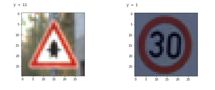
If you are curious, you can always convert an array representation of an image to an image, and see the how it actually looks like. The following code snippets show how you can convert an array back to an image.
Sample image from the Train dataset
# Sample image from the Train dataset # Sample image from Street View Sample
index = 36 index = 24
plt.imshow(X_train[index]) plt.imshow(X_sv_test[index])
print ("y = " + str(np.squeeze(Y_train_orig[index]))) print ("y = " + str(np.squeeze(Y_sv_test_orig[index])))
Setting up Commonly Used Functions
We realized that there are tasks that required us to follow almost the same procedure with slight adjustments to the code. From a programming perspective, this is an area where the usage of functions come in handy. We coded up three functions to encapsulate three tasks: 1) Training and Plotting; 2) Plotting; and 3) Evaluation
The following code snippet displays the code blocks used by us. Feel free to make adjustments wherever necessary.
Common Functions
def train_and_plot(model, epochs = 10, batch_size = 64):
train_dataset = tf.data.Dataset.from_tensor_slices((X_train, Y_train)).batch(batch_size)
val_dataset = tf.data.Dataset.from_tensor_slices((X_val, Y_val)).batch(batch_size )
history = model.fit(train_dataset, epochs = epochs, validation_data=val_dataset)
plot(history)
def plot(history):
# Plotting the Accuracy variation
plt.figure(0)
plt.plot(history.history['accuracy'], label='Training Accuracy')
plt.plot(history.history['val_accuracy'], label='Validation Accuracy')
plt.title('Variation of Accuracy')
plt.xlabel('Epochs')
plt.ylabel('Accuracy')
plt.legend()
plt.show()
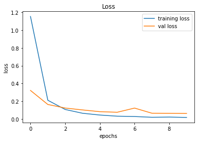
# Plotting the Loss variation
plt.figure(1)
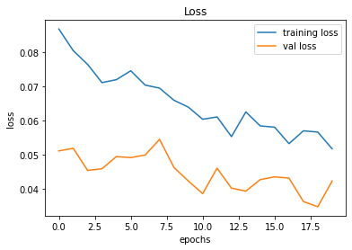
plt.plot(history.history['loss'], label='Training Loss')
plt.plot(history.history['val_loss'], label='Validation Loss')
plt.title('Loss')
plt.xlabel('Epochs')
plt.ylabel('Loss')
plt.legend()
plt.show()
def evaluate_validation(model, no_of_images, rows, columns, dataset_type):
X_ds = None
Y_ds = None
Y_orig_ds = None
result_title = None
if dataset_type == 'test':
X_ds = X_test
Y_ds = Y_test
Y_orig_ds = Y_test_orig
result_title = "TEST"
elif dataset_type == 'val':
X_ds = X_val
Y_ds = Y_val
Y_orig_ds = Y_val_orig
result_title = "VALIDATION"
else:
X_ds = X_sv_test
Y_ds = Y_sv_test
Y_orig_ds = Y_sv_test_orig
result_title = "STREETVIEW TEST"
eval_result = model.evaluate(X_ds, Y_ds)
pred = model.predict(X_ds)
pred_label = [np.argmax(x) for x in pred]
plt.figure(figsize=(25, 25))
for i in range(no_of_images):
plt.subplot(rows, columns, i + 1)
if (pred_label[i] == Y_orig_ds[i]):
plt.title(str(pred_label[i]) + " - CORRECT")
else:
plt.title(str(pred_label[i]) + " - INCORRECT")
plt.imshow(X_ds[i])
plt.axis("off")
plt.show()
y_actu = pd.Series(Y_orig_ds, name='Actual')
y_pred = pd.Series(pred_label, name='Predicted')
conf_matrix = pd.crosstab(y_actu, y_pred)
print(conf_matrix)
accuracy = np.diag(conf_matrix).sum() / conf_matrix.to_numpy().sum()
print("######################")
print(result_title + " Accuracy: " + str(round(eval_result[1],4)*100) + "%")
print("######################")
Model Development - The Iterative Cycle
This will be the longest section of the article as we attempt to explain the thought process behind each tried and tested model. For each model, we will try to be as descriptive as possible and the corresponding results of each model, will also be shown in this section itself (rather than using a different section for Results).
In this section, you will be guided through the process followed by us in implementing and improving the models in an iterative manner. Since this is an iterative procedure, the model accuracy was considered as the single number evaluation metric, and the improvements/modifications are made to models based on the result of the model accuracy obtained by evaluating the validation dataset.
Model 001
The initial model was created to represent the most basic neural network with Input > Dense where we used Adam as the optimizer.
def convolutional_model(input_shape):
input_img = tf.keras.Input(shape=input_shape)
F = tf.keras.layers.Flatten()(input_img)
outputs = tf.keras.layers.Dense(units = 43, activation = 'softmax')(F)
model = tf.keras.Model(inputs=input_img, outputs=outputs)
return model
conv_model_v1 = convolutional_model((30, 30, 3))
conv_model_v1.compile(optimizer='adam',
loss='categorical_crossentropy',
metrics=['accuracy'])
conv_model_v1.summary()
train_and_plot(conv_model_v1)
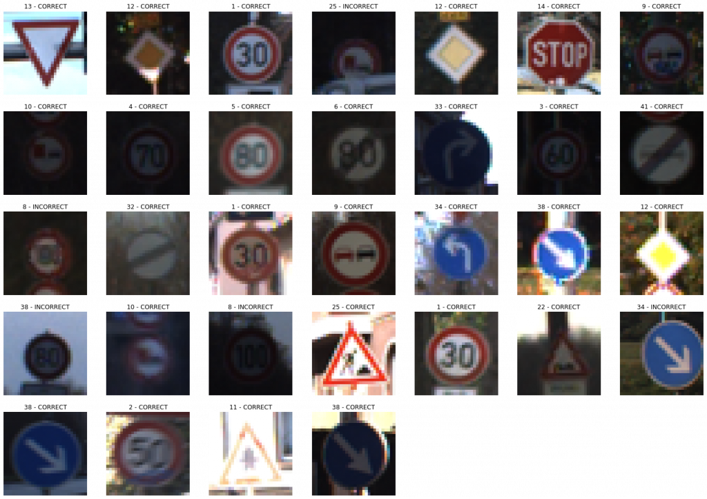
evaluate_validation(model = conv_model_v1, no_of_images = 32, rows = 7, columns = 7, type = 'val')Upon training and plotting, the following outcome was obtained. As it turned out, a validation accuracy of 90.16% was achieved. For a basic neural network, this was an excellent result.
Training and Plotting Results - Model 001

Epoch 1/10
491/491 [==============================] - 2s 4ms/step - loss: 2.0973 - accuracy: 0.5373 - val_loss: 1.4628 - val_accuracy: 0.7042
Epoch 2/10
491/491 [==============================] - 2s 3ms/step - loss: 1.2372 - accuracy: 0.7553 - val_loss: 1.0785 - val_accuracy: 0.7844
Epoch 3/10
491/491 [==============================] - 2s 3ms/step - loss: 0.9560 - accuracy: 0.8221 - val_loss: 0.8889 - val_accuracy: 0.8213
Epoch 4/10
491/491 [==============================] - 2s 3ms/step - loss: 0.7964 - accuracy: 0.8552 - val_loss: 0.7673 - val_accuracy: 0.8475
Epoch 5/10
491/491 [==============================] - 2s 3ms/step - loss: 0.6903 - accuracy: 0.8755 - val_loss: 0.6821 - val_accuracy: 0.8671
Epoch 6/10
491/491 [==============================] - 2s 3ms/step - loss: 0.6133 - accuracy: 0.8893 - val_loss: 0.6203 - val_accuracy: 0.8795
Epoch 7/10
491/491 [==============================] - 2s 3ms/step - loss: 0.5540 - accuracy: 0.8992 - val_loss: 0.5724 - val_accuracy: 0.8898
Epoch 8/10
491/491 [==============================] - 2s 3ms/step - loss: 0.5067 - accuracy: 0.9078 - val_loss: 0.5360 - val_accuracy: 0.8949
Epoch 9/10
491/491 [==============================] - 2s 3ms/step - loss: 0.4680 - accuracy: 0.9141 - val_loss: 0.5084 - val_accuracy: 0.8999
Epoch 10/10
491/491 [==============================] - 2s 3ms/step - loss: 0.4354 - accuracy: 0.9195 - val_loss: 0.4859 - val_accuracy: 0.9016
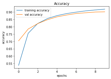
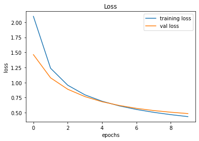
246/246 [==============================] - 0s 2ms/step - loss: 0.4859 - accuracy: 0.9016
######################
VALIDATION Accuracy: 90.16%
######################
Model 002
In this model, the Model 001 is improved by adding a convolutional layer.
def convolutional_model(input_shape):
input_img = tf.keras.Input(shape=input_shape)
Z1 = tf.keras.layers.Conv2D(filters=32, kernel_size= (5, 5), activation = 'relu')(input_img)
F = tf.keras.layers.Flatten()(Z1)
outputs = tf.keras.layers.Dense(units = 43, activation = 'softmax')(F)
model = tf.keras.Model(inputs=input_img, outputs=outputs)
return model
conv_model_v2 = convolutional_model((30, 30, 3))
conv_model_v2.compile(optimizer='adam',
loss='categorical_crossentropy',
metrics=['accuracy'])
conv_model_v2.summary()
train_and_plot(conv_model_v2, epochs = 10)
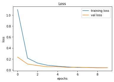
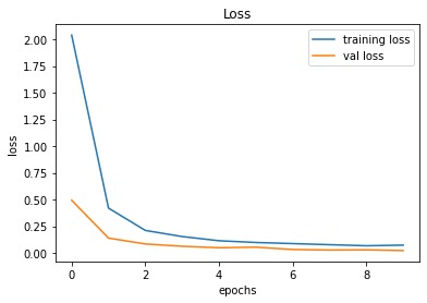
evaluate_validation(model = conv_model_v2, no_of_images = 49, rows = 7, columns = 7, type = 'val')After training, the validation accuracy was increased by the model up to 97.13%. Can we improve it further?
Validation Accuracy of Model 001 = 90.16%Validation Accuracy of Model 002 = 97.13%
Training and Plotting Results - Model 002

Epoch 1/10
491/491 [==============================] - 14s 29ms/step - loss: 0.8728 - accuracy: 0.7880 - val_loss: 0.3256 - val_accuracy: 0.9299
Epoch 2/10
491/491 [==============================] - 14s 29ms/step - loss: 0.2117 - accuracy: 0.9495 - val_loss: 0.2012 - val_accuracy: 0.9569
Epoch 3/10
491/491 [==============================] - 14s 28ms/step - loss: 0.1183 - accuracy: 0.9723 - val_loss: 0.1655 - val_accuracy: 0.9647
Epoch 4/10
491/491 [==============================] - 14s 29ms/step - loss: 0.0850 - accuracy: 0.9796 - val_loss: 0.1794 - val_accuracy: 0.9588
Epoch 5/10
491/491 [==============================] - 14s 29ms/step - loss: 0.0725 - accuracy: 0.9821 - val_loss: 0.1592 - val_accuracy: 0.9663
Epoch 6/10
491/491 [==============================] - 14s 29ms/step - loss: 0.0491 - accuracy: 0.9869 - val_loss: 0.1543 - val_accuracy: 0.9644
Epoch 7/10
491/491 [==============================] - 15s 30ms/step - loss: 0.0519 - accuracy: 0.9866 - val_loss: 0.1247 - val_accuracy: 0.9748
Epoch 8/10
491/491 [==============================] - 14s 29ms/step - loss: 0.0389 - accuracy: 0.9898 - val_loss: 0.1205 - val_accuracy: 0.9773
Epoch 9/10
491/491 [==============================] - 14s 29ms/step - loss: 0.0301 - accuracy: 0.9928 - val_loss: 0.1227 - val_accuracy: 0.9773
Epoch 10/10
491/491 [==============================] - 15s 30ms/step - loss: 0.0271 - accuracy: 0.9930 - val_loss: 0.1390 - val_accuracy: 0.9713
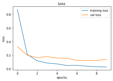
246/246 [==============================] - 1s 6ms/step - loss: 0.1390 - accuracy: 0.9713
Model 003
This is an attempted improvement from Model 002 by adding a MaxPool2D layer.
def convolutional_model(input_shape):
input_img = tf.keras.Input(shape=input_shape)
Z1 = tf.keras.layers.Conv2D(filters=32, kernel_size= (5, 5), activation = 'relu')(input_img)
P1 = tf.keras.layers.MaxPool2D(pool_size=(2, 2))(Z1)
F = tf.keras.layers.Flatten()(P1)
outputs = tf.keras.layers.Dense(units = 43, activation = 'softmax')(F)
model = tf.keras.Model(inputs=input_img, outputs=outputs)
return model
conv_model_v3 = convolutional_model((30, 30, 3))
conv_model_v3.compile(optimizer='adam',
loss='categorical_crossentropy',
metrics=['accuracy'])
conv_model_v3.summary()
train_and_plot(conv_model_v3, epochs = 10)
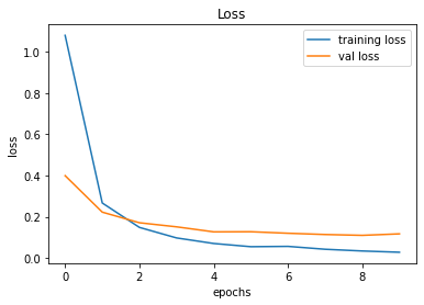
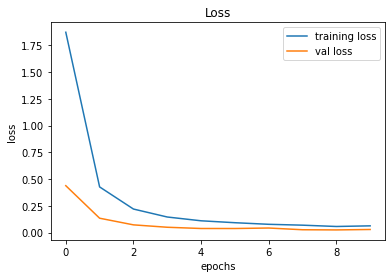
evaluate_validation(model = conv_model_v3, no_of_images = 49, rows = 7, columns = 7, type = 'val')The results between Model 002 and Model 003 are similar. However, there's a noticeable difference between the Training Error and Validation Error and this is an indication of overfitting.
Validation Accuracy of Model 002 = 97.13%Validation Accuracy of Model 003 = 97.45%
Training and Plotting Results - Model 003

Epoch 1/10
491/491 [==============================] - 15s 30ms/step - loss: 1.0802 - accuracy: 0.7429 - val_loss: 0.3993 - val_accuracy: 0.9161
Epoch 2/10
491/491 [==============================] - 15s 30ms/step - loss: 0.2667 - accuracy: 0.9440 - val_loss: 0.2223 - val_accuracy: 0.9510
Epoch 3/10
491/491 [==============================] - 15s 31ms/step - loss: 0.1482 - accuracy: 0.9693 - val_loss: 0.1708 - val_accuracy: 0.9610
Epoch 4/10
491/491 [==============================] - 15s 30ms/step - loss: 0.0971 - accuracy: 0.9806 - val_loss: 0.1510 - val_accuracy: 0.9648
Epoch 5/10
491/491 [==============================] - 16s 32ms/step - loss: 0.0702 - accuracy: 0.9862 - val_loss: 0.1266 - val_accuracy: 0.9727
Epoch 6/10
491/491 [==============================] - 15s 32ms/step - loss: 0.0546 - accuracy: 0.9887 - val_loss: 0.1272 - val_accuracy: 0.9709
Epoch 7/10
491/491 [==============================] - 16s 33ms/step - loss: 0.0561 - accuracy: 0.9885 - val_loss: 0.1198 - val_accuracy: 0.9754
Epoch 8/10
491/491 [==============================] - 15s 31ms/step - loss: 0.0422 - accuracy: 0.9911 - val_loss: 0.1137 - val_accuracy: 0.9770
Epoch 9/10
491/491 [==============================] - 15s 31ms/step - loss: 0.0338 - accuracy: 0.9925 - val_loss: 0.1097 - val_accuracy: 0.9762
Epoch 10/10
491/491 [==============================] - 16s 32ms/step - loss: 0.0277 - accuracy: 0.9942 - val_loss: 0.1169 - val_accuracy: 0.9745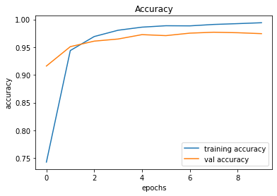
246/246 [==============================] - 1s 6ms/step - loss: 0.1169 - accuracy: 0.9745
Model 004
We will add another Convolutional Layer too see if the results improve to minimize the bias (before focusing on the overfitting problems).
def convolutional_model(input_shape):
input_img = tf.keras.Input(shape=input_shape)
Z1 = tf.keras.layers.Conv2D(filters=32, kernel_size= (5, 5), activation = 'relu')(input_img)
P1 = tf.keras.layers.MaxPool2D(pool_size=(2, 2))(Z1)
Z2 = tf.keras.layers.Conv2D(filters=64, kernel_size= (5, 5), activation = 'relu')(P1)
F = tf.keras.layers.Flatten()(Z2)
outputs = tf.keras.layers.Dense(units = 43, activation = 'softmax')(F)
model = tf.keras.Model(inputs=input_img, outputs=outputs)
return model
conv_model_v4 = convolutional_model((30, 30, 3))
conv_model_v4.compile(optimizer='adam',
loss='categorical_crossentropy',
metrics=['accuracy'])
conv_model_v4.summary()
train_and_plot(conv_model_v4, epochs = 10)
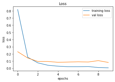
evaluate_validation(model = conv_model_4, no_of_images = 49, rows = 7, columns = 7, type = 'val')While the validation accuracy improved by approximately 1%, the overfitting problem remains an issue due to the difference between the Training Error and Validation Error.
Validation Accuracy of Model 003 = 97.45%Validation Accuracy of Model 004 = 98.51%
Training and Plotting Results - Model 004

Epoch 1/10
491/491 [==============================] - 26s 53ms/step - loss: 0.8186 - accuracy: 0.7919 - val_loss: 0.2310 - val_accuracy: 0.9498
Epoch 2/10
491/491 [==============================] - 27s 55ms/step - loss: 0.1544 - accuracy: 0.9647 - val_loss: 0.1435 - val_accuracy: 0.9675
Epoch 3/10
491/491 [==============================] - 30s 60ms/step - loss: 0.0759 - accuracy: 0.9824 - val_loss: 0.0957 - val_accuracy: 0.9800
Epoch 4/10
491/491 [==============================] - 29s 59ms/step - loss: 0.0426 - accuracy: 0.9901 - val_loss: 0.0951 - val_accuracy: 0.9796
Epoch 5/10
491/491 [==============================] - 28s 58ms/step - loss: 0.0297 - accuracy: 0.9926 - val_loss: 0.0839 - val_accuracy: 0.9837
Epoch 6/10
491/491 [==============================] - 28s 56ms/step - loss: 0.0223 - accuracy: 0.9942 - val_loss: 0.0870 - val_accuracy: 0.9813
Epoch 7/10
491/491 [==============================] - 27s 55ms/step - loss: 0.0221 - accuracy: 0.9947 - val_loss: 0.0908 - val_accuracy: 0.9816
Epoch 8/10
491/491 [==============================] - 27s 56ms/step - loss: 0.0247 - accuracy: 0.9931 - val_loss: 0.0877 - val_accuracy: 0.9836
Epoch 9/10
491/491 [==============================] - 27s 56ms/step - loss: 0.0110 - accuracy: 0.9973 - val_loss: 0.1071 - val_accuracy: 0.9821
Epoch 10/10
491/491 [==============================] - 28s 57ms/step - loss: 0.0069 - accuracy: 0.9984 - val_loss: 0.0817 - val_accuracy: 0.9851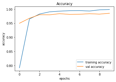
246/246 [==============================] - 2s 8ms/step - loss: 0.0817 - accuracy: 0.9851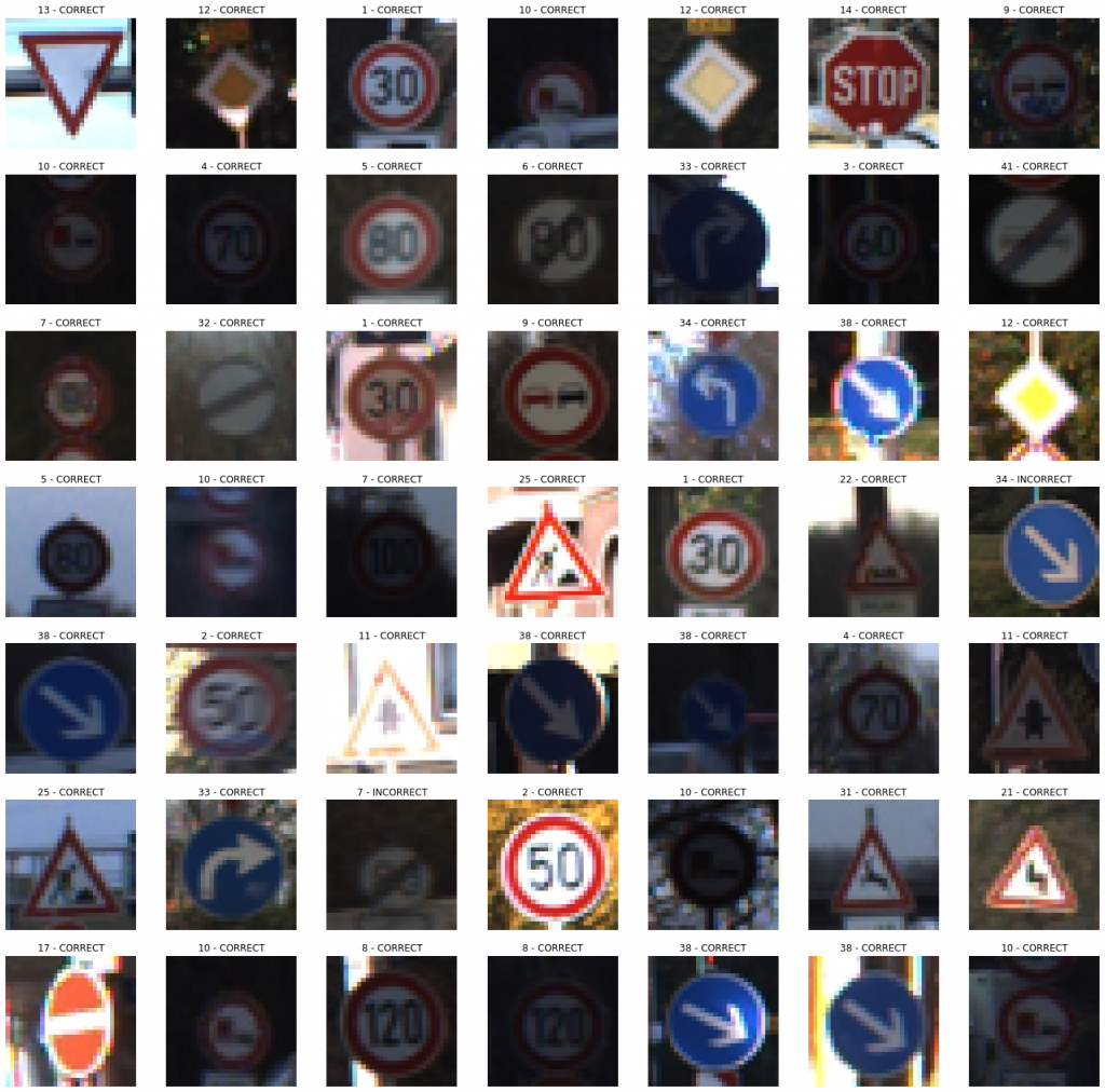
Model 005
We will add another MaxPooling2D Layer before going ahead with the regularization to tackle the overfitting problem.
def convolutional_model(input_shape):
    input_img = tf.keras.Input(shape=input_shape)
    Z1 = tf.keras.layers.Conv2D(filters=32, kernel_size= (5, 5), activation = 'relu')(input_img)
    P1 = tf.keras.layers.MaxPool2D(pool_size=(2, 2))(Z1)
    Z2 = tf.keras.layers.Conv2D(filters=64, kernel_size= (5, 5), activation = 'relu')(P1)
    P2 = tf.keras.layers.MaxPool2D(pool_size=(2, 2))(Z2)
    F = tf.keras.layers.Flatten()(P2)
    outputs = tf.keras.layers.Dense(units = 43, activation = 'softmax')(F)
    model = tf.keras.Model(inputs=input_img, outputs=outputs)
    return model

conv_model_v5 = convolutional_model((30, 30, 3))
conv_model_v5.compile(optimizer='adam',
                  loss='categorical_crossentropy',
                  metrics=['accuracy'])
conv_model_v5.summary()
train_and_plot(conv_model_v8, epochs = 10)
There is a slight improvement in the validation accuracy from 98.51% to 98.83%. However, there is still a slight difference between the training and validation accuracies.
Validation Accuracy of Model 004 = 98.51%Validation Accuracy of Model 005 = 98.83%
Training and Plotting Results - Model 005

Epoch 1/10
491/491 [==============================] - 25s 51ms/step - loss: 1.1546 - accuracy: 0.7134 - val_loss: 0.3212 - val_accuracy: 0.9245
Epoch 2/10
491/491 [==============================] - 25s 50ms/step - loss: 0.2106 - accuracy: 0.9515 - val_loss: 0.1631 - val_accuracy: 0.9611
Epoch 3/10
491/491 [==============================] - 26s 53ms/step - loss: 0.1069 - accuracy: 0.9764 - val_loss: 0.1229 - val_accuracy: 0.9697
Epoch 4/10
491/491 [==============================] - 26s 54ms/step - loss: 0.0641 - accuracy: 0.9858 - val_loss: 0.1016 - val_accuracy: 0.9749
Epoch 5/10
491/491 [==============================] - 27s 54ms/step - loss: 0.0441 - accuracy: 0.9908 - val_loss: 0.0819 - val_accuracy: 0.9815
Epoch 6/10
491/491 [==============================] - 26s 54ms/step - loss: 0.0311 - accuracy: 0.9936 - val_loss: 0.0754 - val_accuracy: 0.9829
Epoch 7/10
491/491 [==============================] - 27s 55ms/step - loss: 0.0274 - accuracy: 0.9935 - val_loss: 0.1225 - val_accuracy: 0.9750
Epoch 8/10
491/491 [==============================] - 26s 53ms/step - loss: 0.0188 - accuracy: 0.9956 - val_loss: 0.0646 - val_accuracy: 0.9846
Epoch 9/10
491/491 [==============================] - 25s 51ms/step - loss: 0.0211 - accuracy: 0.9951 - val_loss: 0.0637 - val_accuracy: 0.9866
Epoch 10/10
491/491 [==============================] - 25s 51ms/step - loss: 0.0170 - accuracy: 0.9960 - val_loss: 0.0621 - val_accuracy: 0.9883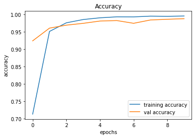
246/246 [==============================] - 2s 8ms/step - loss: 0.0621 - accuracy: 0.9883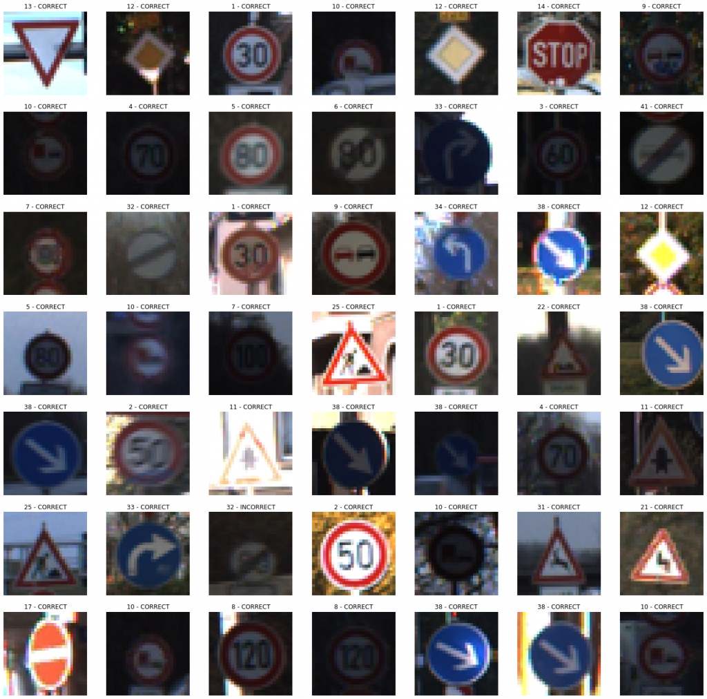
Model 006
Because of the difference between the training and validation accuracies, we are now adding a Dropout layer to address the overfitting problem.
def convolutional_model(input_shape):
    input_img = tf.keras.Input(shape=input_shape)
    Z1 = tf.keras.layers.Conv2D(filters=32, kernel_size= (5, 5), activation = 'relu')(input_img)
    P1 = tf.keras.layers.MaxPool2D(pool_size=(2, 2))(Z1)
    D1 = tf.keras.layers.Dropout(rate = 0.25)(P1)
    Z2 = tf.keras.layers.Conv2D(filters=64, kernel_size= (5, 5), activation = 'relu')(D1)
    P2 = tf.keras.layers.MaxPool2D(pool_size=(2, 2))(Z2)
    F = tf.keras.layers.Flatten()(P2)
    outputs = tf.keras.layers.Dense(units = 43, activation = 'softmax')(F)
    model = tf.keras.Model(inputs=input_img, outputs=outputs)
    return model

conv_model_v6 = convolutional_model((30, 30, 3))
conv_model_v6.compile(optimizer='adam',
                  loss='categorical_crossentropy',
                  metrics=['accuracy'])
conv_model_v6.summary()
train_and_plot(conv_model_v6, epochs = 10)
evaluate_validation(model = conv_model_v6, no_of_images = 49, rows = 7, columns = 7, type = 'val')
The Dropout certainly had an effect in narrowing down the gap between Training Error and Validation Error. However, there is an indication of validation accuracy going down after Epoch 09. In such cases, Early Stopping may come in handy.
Validation Accuracy of Model 005 = 98.83%Validation Accuracy of Model 006 = 98.83%
Training and Plotting Results - Model 006

Epoch 1/10
491/491 [==============================] - 29s 59ms/step - loss: 1.2292 - accuracy: 0.6867 - val_loss: 0.3695 - val_accuracy: 0.9115
Epoch 2/10
491/491 [==============================] - 29s 59ms/step - loss: 0.2606 - accuracy: 0.9351 - val_loss: 0.1708 - val_accuracy: 0.9634
Epoch 3/10
491/491 [==============================] - 30s 62ms/step - loss: 0.1393 - accuracy: 0.9661 - val_loss: 0.1292 - val_accuracy: 0.9686
Epoch 4/10
491/491 [==============================] - 30s 61ms/step - loss: 0.0874 - accuracy: 0.9791 - val_loss: 0.0912 - val_accuracy: 0.9802
Epoch 5/10
491/491 [==============================] - 29s 59ms/step - loss: 0.0680 - accuracy: 0.9835 - val_loss: 0.0797 - val_accuracy: 0.9815
Epoch 6/10
491/491 [==============================] - 29s 59ms/step - loss: 0.0496 - accuracy: 0.9882 - val_loss: 0.0736 - val_accuracy: 0.9847
Epoch 7/10
491/491 [==============================] - 30s 60ms/step - loss: 0.0411 - accuracy: 0.9896 - val_loss: 0.0669 - val_accuracy: 0.9846
Epoch 8/10
491/491 [==============================] - 29s 60ms/step - loss: 0.0362 - accuracy: 0.9899 - val_loss: 0.0481 - val_accuracy: 0.9894
Epoch 9/10
491/491 [==============================] - 30s 60ms/step - loss: 0.0285 - accuracy: 0.9928 - val_loss: 0.0496 - val_accuracy: 0.9888
Epoch 10/10
491/491 [==============================] - 30s 61ms/step - loss: 0.0259 - accuracy: 0.9936 - val_loss: 0.0557 - val_accuracy: 0.9883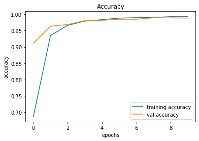
246/246 [==============================] - 2s 8ms/step - loss: 0.0557 - accuracy: 0.9883
Model 007
We will add another Dropout layer to see if we can further fine-tune the model and then let's proceed with Early Stopping if necessary.
# Model 007
def convolutional_model(input_shape):
input_img = tf.keras.Input(shape=input_shape)
Z1 = tf.keras.layers.Conv2D(filters=32, kernel_size= (5, 5), activation = 'relu')(input_img)
P1 = tf.keras.layers.MaxPool2D(pool_size=(2, 2))(Z1)
D1 = tf.keras.layers.Dropout(rate = 0.25)(P1)
Z2 = tf.keras.layers.Conv2D(filters=64, kernel_size= (5, 5), activation = 'relu')(D1)
P2 = tf.keras.layers.MaxPool2D(pool_size=(2, 2))(Z2)
D2 = tf.keras.layers.Dropout(rate = 0.25)(P2)
F = tf.keras.layers.Flatten()(D2)
outputs = tf.keras.layers.Dense(units = 43, activation = 'softmax')(F)
model = tf.keras.Model(inputs=input_img, outputs=outputs)
return model
conv_model_v7 = convolutional_model((30, 30, 3))
conv_model_v7.compile(optimizer='adam',
loss='categorical_crossentropy',
metrics=['accuracy'])
conv_model_v7.summary()
train_and_plot(conv_model_v7, epochs = 10)
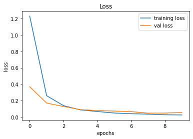
evaluate_validation(model = conv_model_v7, no_of_images = 49, rows = 7, columns = 7, type = 'val')The validation accuracy slightly improved from 98.83% to 99.22%.
Validation Accuracy of Model 006 = 98.83%Validation Accuracy of Model 007 = 99.22%
Training and Plotting Results - Model 007

Epoch 1/10
491/491 [==============================] - 30s 61ms/step - loss: 1.3423 - accuracy: 0.6474 - val_loss: 0.3653 - val_accuracy: 0.9217
Epoch 2/10
491/491 [==============================] - 30s 62ms/step - loss: 0.3166 - accuracy: 0.9155 - val_loss: 0.1653 - val_accuracy: 0.9675
Epoch 3/10
491/491 [==============================] - 31s 64ms/step - loss: 0.1760 - accuracy: 0.9539 - val_loss: 0.1124 - val_accuracy: 0.9784
Epoch 4/10
491/491 [==============================] - 36s 74ms/step - loss: 0.1198 - accuracy: 0.9687 - val_loss: 0.0857 - val_accuracy: 0.9844
Epoch 5/10
491/491 [==============================] - 39s 80ms/step - loss: 0.0861 - accuracy: 0.9769 - val_loss: 0.0709 - val_accuracy: 0.9837
Epoch 6/10
491/491 [==============================] - 32s 66ms/step - loss: 0.0710 - accuracy: 0.9808 - val_loss: 0.0517 - val_accuracy: 0.9892
Epoch 7/10
491/491 [==============================] - 41s 84ms/step - loss: 0.0621 - accuracy: 0.9830 - val_loss: 0.0535 - val_accuracy: 0.9895
Epoch 8/10
491/491 [==============================] - 34s 68ms/step - loss: 0.0486 - accuracy: 0.9868 - val_loss: 0.0422 - val_accuracy: 0.9922
Epoch 9/10
491/491 [==============================] - 30s 61ms/step - loss: 0.0424 - accuracy: 0.9881 - val_loss: 0.0458 - val_accuracy: 0.9903
Epoch 10/10
491/491 [==============================] - 30s 62ms/step - loss: 0.0416 - accuracy: 0.9881 - val_loss: 0.0387 - val_accuracy: 0.9922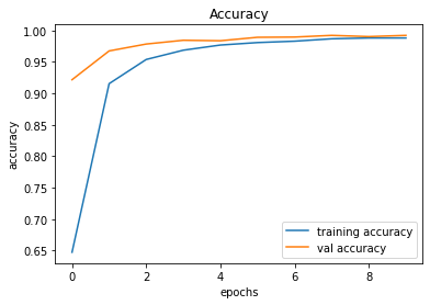
246/246 [==============================] - 2s 8ms/step - loss: 0.0387 - accuracy: 0.9922
Model 008
Adding more layers make the network deeper and having a bigger network almost always helps in minimizing the bias, and for increasing the accuracy. Therefore, we will add another Convolutional Layer to see if we can further increase the Validation Accuracy. On the other hand, the validation accuracy surpassed the training accuracy, and this happens due to the effect of Dropout.
def convolutional_model(input_shape):
input_img = tf.keras.Input(shape=input_shape)
Z1 = tf.keras.layers.Conv2D(filters=32, kernel_size= (5, 5), activation = 'relu')(input_img)
P1 = tf.keras.layers.MaxPool2D(pool_size=(2, 2))(Z1)
D1 = tf.keras.layers.Dropout(rate = 0.25)(P1)
Z2 = tf.keras.layers.Conv2D(filters=64, kernel_size= (5, 5), activation = 'relu')(D1)
P2 = tf.keras.layers.MaxPool2D(pool_size=(2, 2))(Z2)
D2 = tf.keras.layers.Dropout(rate = 0.25)(P2)
Z3 = tf.keras.layers.Conv2D(filters=256, kernel_size= (3, 3), activation = 'relu')(D2)
F = tf.keras.layers.Flatten()(Z3)
outputs = tf.keras.layers.Dense(units = 43, activation = 'softmax')(F)
model = tf.keras.Model(inputs=input_img, outputs=outputs)
return model
conv_model_v8 = convolutional_model((30, 30, 3))
conv_model_v8.compile(optimizer='adam',
loss='categorical_crossentropy',
metrics=['accuracy'])
conv_model_v8.summary()
train_and_plot(conv_model_v8, epochs = 10)
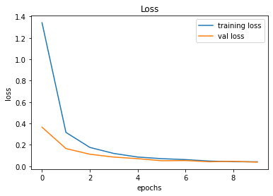
evaluate_validation(model = conv_model_v8, no_of_images = 49, rows = 7, columns = 7, type = 'val')The validation accuracy slightly improved from 99.22% to 99.34%.
Validation Accuracy of Model 007 = 98.22%Validation Accuracy of Model 008 = 99.34%
Training and Plotting Results - Model 008
Epoch 1/10
491/491 [==============================] - 31s 63ms/step - loss: 1.1019 - accuracy: 0.6988 - val_loss: 0.2339 - val_accuracy: 0.9439
Epoch 2/10
491/491 [==============================] - 32s 65ms/step - loss: 0.2157 - accuracy: 0.9404 - val_loss: 0.1071 - val_accuracy: 0.9740
Epoch 3/10
491/491 [==============================] - 35s 72ms/step - loss: 0.1245 - accuracy: 0.9656 - val_loss: 0.0783 - val_accuracy: 0.9830
Epoch 4/10
491/491 [==============================] - 33s 67ms/step - loss: 0.0837 - accuracy: 0.9761 - val_loss: 0.0574 - val_accuracy: 0.9892
Epoch 5/10
491/491 [==============================] - 34s 70ms/step - loss: 0.0669 - accuracy: 0.9806 - val_loss: 0.0595 - val_accuracy: 0.9884
Epoch 6/10
491/491 [==============================] - 33s 68ms/step - loss: 0.0540 - accuracy: 0.9848 - val_loss: 0.0446 - val_accuracy: 0.9926
Epoch 7/10
491/491 [==============================] - 35s 71ms/step - loss: 0.0424 - accuracy: 0.9877 - val_loss: 0.0486 - val_accuracy: 0.9899
Epoch 8/10
491/491 [==============================] - 33s 68ms/step - loss: 0.0447 - accuracy: 0.9868 - val_loss: 0.0429 - val_accuracy: 0.9911
Epoch 9/10
491/491 [==============================] - 36s 73ms/step - loss: 0.0405 - accuracy: 0.9879 - val_loss: 0.0373 - val_accuracy: 0.9930
Epoch 10/10
491/491 [==============================] - 38s 78ms/step - loss: 0.0393 - accuracy: 0.9881 - val_loss: 0.0392 - val_accuracy: 0.9934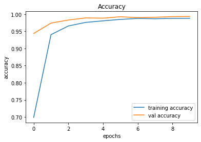
246/246 [==============================] - 2s 10ms/step - loss: 0.0392 - accuracy: 0.9934
Model 009
We further add another MaxPool2D layer, followed by a Dropout layer.
def convolutional_model(input_shape):
    input_img = tf.keras.Input(shape=input_shape)
    Z1 = tf.keras.layers.Conv2D(filters=32, kernel_size= (5, 5), activation = 'relu')(input_img)
    P1 = tf.keras.layers.MaxPool2D(pool_size=(2, 2))(Z1)
    D1 = tf.keras.layers.Dropout(rate = 0.25)(P1)
    Z2 = tf.keras.layers.Conv2D(filters=64, kernel_size= (5, 5), activation = 'relu')(D1)
    P2 = tf.keras.layers.MaxPool2D(pool_size=(2, 2))(Z2)
    D2 = tf.keras.layers.Dropout(rate = 0.25)(P2)
    Z3 = tf.keras.layers.Conv2D(filters=256, kernel_size= (3, 3), activation = 'relu')(D2)
    P3 = tf.keras.layers.MaxPool2D(pool_size=(2, 2))(Z3)
    D3 = tf.keras.layers.Dropout(rate = 0.25)(P3)
    F = tf.keras.layers.Flatten()(D3)
    outputs = tf.keras.layers.Dense(units = 43, activation = 'softmax')(F)
    model = tf.keras.Model(inputs=input_img, outputs=outputs)
    return model

conv_model_v9 = convolutional_model((30, 30, 3))
conv_model_v9.compile(optimizer='adam',
                  loss='categorical_crossentropy',
                  metrics=['accuracy'])
conv_model_v9.summary()
train_and_plot(conv_model_v9, epochs = 10)
evaluate_validation(model = conv_model_v9, no_of_images = 49, rows = 7, columns = 7, type = 'val')
The validation accuracy slightly improved from 99.34% to 99.36%.
Validation Accuracy of Model 008 = 98.34%Validation Accuracy of Model 009 = 99.36%Training and Plotting Result - Model 009
Training and Plotting Results - Model 009

Epoch 1/10
491/491 [==============================] - 32s 64ms/step - loss: 1.8729 - accuracy: 0.4747 - val_loss: 0.4384 - val_accuracy: 0.8979
Epoch 2/10
491/491 [==============================] - 33s 66ms/step - loss: 0.4269 - accuracy: 0.8749 - val_loss: 0.1343 - val_accuracy: 0.9718
Epoch 3/10
491/491 [==============================] - 34s 69ms/step - loss: 0.2201 - accuracy: 0.9376 - val_loss: 0.0722 - val_accuracy: 0.9852
Epoch 4/10
491/491 [==============================] - 34s 69ms/step - loss: 0.1456 - accuracy: 0.9567 - val_loss: 0.0498 - val_accuracy: 0.9895
Epoch 5/10
491/491 [==============================] - 34s 69ms/step - loss: 0.1102 - accuracy: 0.9676 - val_loss: 0.0382 - val_accuracy: 0.9926
Epoch 6/10
491/491 [==============================] - 34s 70ms/step - loss: 0.0923 - accuracy: 0.9729 - val_loss: 0.0380 - val_accuracy: 0.9932
Epoch 7/10
491/491 [==============================] - 34s 69ms/step - loss: 0.0773 - accuracy: 0.9774 - val_loss: 0.0426 - val_accuracy: 0.9902
Epoch 8/10
491/491 [==============================] - 33s 67ms/step - loss: 0.0692 - accuracy: 0.9800 - val_loss: 0.0265 - val_accuracy: 0.9943
Epoch 9/10
491/491 [==============================] - 32s 66ms/step - loss: 0.0570 - accuracy: 0.9839 - val_loss: 0.0249 - val_accuracy: 0.9939
Epoch 10/10
491/491 [==============================] - 32s 65ms/step - loss: 0.0630 - accuracy: 0.9807 - val_loss: 0.0290 - val_accuracy: 0.9936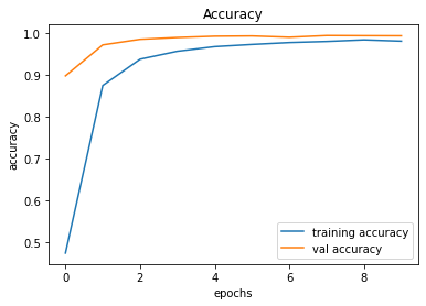
Model 010
Now, we will add a Fully Connected Layer to see if it improves the overall performance (and minimize the bias).
def convolutional_model(input_shape):
    input_img = tf.keras.Input(shape=input_shape)
    Z1 = tf.keras.layers.Conv2D(filters=32, kernel_size= (5, 5), activation = 'relu')(input_img)
    P1 = tf.keras.layers.MaxPool2D(pool_size=(2, 2))(Z1)
    D1 = tf.keras.layers.Dropout(rate = 0.25)(P1)
    Z2 = tf.keras.layers.Conv2D(filters=64, kernel_size= (5, 5), activation = 'relu')(D1)
    P2 = tf.keras.layers.MaxPool2D(pool_size=(2, 2))(Z2)
    D2 = tf.keras.layers.Dropout(rate = 0.25)(P2)
    Z3 = tf.keras.layers.Conv2D(filters=256, kernel_size= (3, 3), activation = 'relu')(D2)
    P3 = tf.keras.layers.MaxPool2D(pool_size=(2, 2))(Z3)
    D3 = tf.keras.layers.Dropout(rate = 0.25)(P3)
    F = tf.keras.layers.Flatten()(D3)
    FC1 = tf.keras.layers.Dense(units = 256, activation = 'relu')(F)
    outputs = tf.keras.layers.Dense(units = 43, activation = 'softmax')(FC1)
    model = tf.keras.Model(inputs=input_img, outputs=outputs)
    return model

conv_model_v10 = convolutional_model((30, 30, 3))
conv_model_v10.compile(optimizer='adam',
                  loss='categorical_crossentropy',
                  metrics=['accuracy'])
conv_model_v10.summary()
train_and_plot(conv_model_v10, epochs = 10)
Validation Accuracy of Model 009 = 98.36%Validation Accuracy of Model 010 = 99.38%
Training and Plotting Results - Model 010

Epoch 1/10
491/491 [==============================] - 31s 63ms/step - loss: 2.0385 - accuracy: 0.4115 - val_loss: 0.4938 - val_accuracy: 0.8601
Epoch 2/10
491/491 [==============================] - 31s 63ms/step - loss: 0.4200 - accuracy: 0.8677 - val_loss: 0.1395 - val_accuracy: 0.9675
Epoch 3/10
491/491 [==============================] - 32s 66ms/step - loss: 0.2112 - accuracy: 0.9377 - val_loss: 0.0846 - val_accuracy: 0.9793
Epoch 4/10
491/491 [==============================] - 32s 65ms/step - loss: 0.1538 - accuracy: 0.9545 - val_loss: 0.0630 - val_accuracy: 0.9856
Epoch 5/10
491/491 [==============================] - 32s 65ms/step - loss: 0.1147 - accuracy: 0.9645 - val_loss: 0.0494 - val_accuracy: 0.9878
Epoch 6/10
491/491 [==============================] - 32s 65ms/step - loss: 0.0984 - accuracy: 0.9698 - val_loss: 0.0545 - val_accuracy: 0.9858
Epoch 7/10
491/491 [==============================] - 32s 66ms/step - loss: 0.0881 - accuracy: 0.9729 - val_loss: 0.0326 - val_accuracy: 0.9918
Epoch 8/10
491/491 [==============================] - 32s 65ms/step - loss: 0.0778 - accuracy: 0.9764 - val_loss: 0.0275 - val_accuracy: 0.9935
Epoch 9/10
491/491 [==============================] - 32s 65ms/step - loss: 0.0679 - accuracy: 0.9787 - val_loss: 0.0291 - val_accuracy: 0.9920
Epoch 10/10
491/491 [==============================] - 32s 66ms/step - loss: 0.0736 - accuracy: 0.9782 - val_loss: 0.0226 - val_accuracy: 0.9938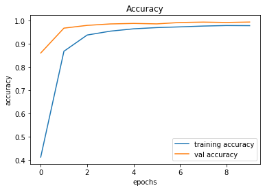
246/246 [==============================] - 2s 9ms/step - loss: 0.0226 - accuracy: 0.9938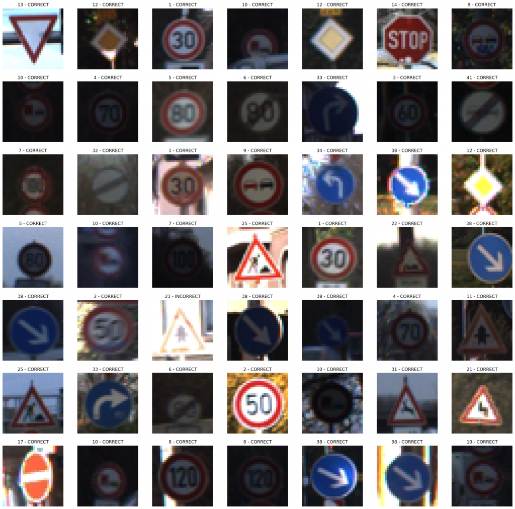
Model 011
While it may not have a considerable effect, it is worth a try to add a regularizer to the Fully Connected Layer.
def convolutional_model(input_shape):
    input_img = tf.keras.Input(shape=input_shape)
    Z1 = tf.keras.layers.Conv2D(filters=32, kernel_size= (5, 5), activation = 'relu')(input_img)
    P1 = tf.keras.layers.MaxPool2D(pool_size=(2, 2))(Z1)
    D1 = tf.keras.layers.Dropout(rate = 0.25)(P1)
    Z2 = tf.keras.layers.Conv2D(filters=64, kernel_size= (5, 5), activation = 'relu')(D1)
    P2 = tf.keras.layers.MaxPool2D(pool_size=(2, 2))(Z2)
    D2 = tf.keras.layers.Dropout(rate = 0.25)(P2)
    Z3 = tf.keras.layers.Conv2D(filters=256, kernel_size= (3, 3), activation = 'relu')(D2)
    P3 = tf.keras.layers.MaxPool2D(pool_size=(2, 2))(Z3)
    D3 = tf.keras.layers.Dropout(rate = 0.25)(P3)
    F = tf.keras.layers.Flatten()(D3)
    FC1 = tf.keras.layers.Dense(units = 256, activation = 'relu', kernel_regularizer=regularizers.l2(0.0001))(F)
    outputs = tf.keras.layers.Dense(units = 43, activation = 'softmax')(FC1)
    model = tf.keras.Model(inputs=input_img, outputs=outputs)
    return model

conv_model_v11 = convolutional_model((30, 30, 3))
conv_model_v11.compile(optimizer='adam',
                  loss='categorical_crossentropy',
                  metrics=['accuracy'])
conv_model_v11.summary()
train_and_plot(conv_model_v11, epochs = 10)
evaluate_validation(model = conv_model_v11, no_of_images = 49, rows = 7, columns = 7, type = 'val')
Validation Accuracy of Model 010 = 99.38%Validation Accuracy of Model 011 = 99.44%
Epoch 1/10
491/491 [==============================] - 32s 66ms/step - loss: 1.9605 - accuracy: 0.4357 - val_loss: 0.5152 - val_accuracy: 0.8624
Epoch 2/10
491/491 [==============================] - 34s 69ms/step - loss: 0.4549 - accuracy: 0.8630 - val_loss: 0.1577 - val_accuracy: 0.9679
Epoch 3/10
491/491 [==============================] - 33s 67ms/step - loss: 0.2494 - accuracy: 0.9301 - val_loss: 0.1195 - val_accuracy: 0.9779
Epoch 4/10
491/491 [==============================] - 32s 66ms/step - loss: 0.1742 - accuracy: 0.9527 - val_loss: 0.0850 - val_accuracy: 0.9860
Epoch 5/10
491/491 [==============================] - 32s 66ms/step - loss: 0.1446 - accuracy: 0.9633 - val_loss: 0.0758 - val_accuracy: 0.9889
Epoch 6/10
491/491 [==============================] - 33s 66ms/step - loss: 0.1236 - accuracy: 0.9696 - val_loss: 0.0676 - val_accuracy: 0.9908
Epoch 7/10
491/491 [==============================] - 33s 67ms/step - loss: 0.1121 - accuracy: 0.9726 - val_loss: 0.0618 - val_accuracy: 0.9918
Epoch 8/10
491/491 [==============================] - 34s 68ms/step - loss: 0.1026 - accuracy: 0.9765 - val_loss: 0.0585 - val_accuracy: 0.9920
Epoch 9/10
491/491 [==============================] - 32s 66ms/step - loss: 0.0965 - accuracy: 0.9778 - val_loss: 0.0539 - val_accuracy: 0.9926
Epoch 10/10
491/491 [==============================] - 33s 66ms/step - loss: 0.0914 - accuracy: 0.9789 - val_loss: 0.0495 - val_accuracy: 0.9944
246/246 [==============================] - 2s 10ms/step - loss: 0.0495 - accuracy: 0.9944
Since we have achieved an acceptable accuracy, let us try to train longer by increasing the number of epochs. While training longer does not always help, it never hurts to try training longer.
train_and_plot(conv_model_v11, epochs = 20)Validation Accuracy of Model 011 (with 10 epochs) = 99.44%Validation Accuracy of Model 011 (with 20 epochs) = 99.53%
Epoch 1/20
491/491 [==============================] - 30s 62ms/step - loss: 0.0867 - accuracy: 0.9806 - val_loss: 0.0511 - val_accuracy: 0.9939
Epoch 2/20
491/491 [==============================] - 32s 64ms/step - loss: 0.0804 - accuracy: 0.9834 - val_loss: 0.0518 - val_accuracy: 0.9938
Epoch 3/20
491/491 [==============================] - 34s 69ms/step - loss: 0.0764 - accuracy: 0.9835 - val_loss: 0.0454 - val_accuracy: 0.9948
Epoch 4/20
491/491 [==============================] - 32s 65ms/step - loss: 0.0710 - accuracy: 0.9849 - val_loss: 0.0459 - val_accuracy: 0.9943
Epoch 5/20
491/491 [==============================] - 31s 64ms/step - loss: 0.0719 - accuracy: 0.9844 - val_loss: 0.0494 - val_accuracy: 0.9927
Epoch 6/20
491/491 [==============================] - 31s 64ms/step - loss: 0.0745 - accuracy: 0.9837 - val_loss: 0.0491 - val_accuracy: 0.9941
Epoch 7/20
491/491 [==============================] - 32s 65ms/step - loss: 0.0703 - accuracy: 0.9855 - val_loss: 0.0499 - val_accuracy: 0.9939
Epoch 8/20
491/491 [==============================] - 32s 65ms/step - loss: 0.0694 - accuracy: 0.9853 - val_loss: 0.0545 - val_accuracy: 0.9926
Epoch 9/20
491/491 [==============================] - 33s 67ms/step - loss: 0.0659 - accuracy: 0.9865 - val_loss: 0.0463 - val_accuracy: 0.9952
Epoch 10/20
491/491 [==============================] - 33s 67ms/step - loss: 0.0639 - accuracy: 0.9875 - val_loss: 0.0423 - val_accuracy: 0.9952
Epoch 11/20
491/491 [==============================] - 36s 72ms/step - loss: 0.0603 - accuracy: 0.9873 - val_loss: 0.0386 - val_accuracy: 0.9954
Epoch 12/20
491/491 [==============================] - 32s 66ms/step - loss: 0.0610 - accuracy: 0.9871 - val_loss: 0.0460 - val_accuracy: 0.9935
Epoch 13/20
491/491 [==============================] - 30s 61ms/step - loss: 0.0553 - accuracy: 0.9898 - val_loss: 0.0402 - val_accuracy: 0.9963
Epoch 14/20
491/491 [==============================] - 34s 69ms/step - loss: 0.0625 - accuracy: 0.9869 - val_loss: 0.0393 - val_accuracy: 0.9960
Epoch 15/20
491/491 [==============================] - 40s 81ms/step - loss: 0.0584 - accuracy: 0.9877 - val_loss: 0.0427 - val_accuracy: 0.9957
Epoch 16/20
491/491 [==============================] - 42s 86ms/step - loss: 0.0580 - accuracy: 0.9881 - val_loss: 0.0435 - val_accuracy: 0.9955
Epoch 17/20
491/491 [==============================] - 37s 76ms/step - loss: 0.0532 - accuracy: 0.9900 - val_loss: 0.0431 - val_accuracy: 0.9952
Epoch 18/20
491/491 [==============================] - 35s 71ms/step - loss: 0.0570 - accuracy: 0.9889 - val_loss: 0.0363 - val_accuracy: 0.9959
Epoch 19/20
491/491 [==============================] - 34s 69ms/step - loss: 0.0566 - accuracy: 0.9889 - val_loss: 0.0348 - val_accuracy: 0.9969
Epoch 20/20
491/491 [==============================] - 34s 70ms/step - loss: 0.0517 - accuracy: 0.9896 - val_loss: 0.0423 - val_accuracy: 0.9953
246/246 [==============================] - 2s 8ms/step - loss: 0.0423 - accuracy: 0.9953
We will consider this as the final model because we have been able to achieve a validation accuracy of over 99.50%. The following code snippet should assist us in saving the final model in Hierarchical Data Format version 5 (HDF5).
conv_model_v11.save("gtsrb_v11.h5")Summary
The table given below, summarizes the results of the models that we implemented.
The Test Drive
| Model | Accuracy |
| Model 001 | 90.16% |
| Model 002 | 97.13% |
| Model 003 | 97.45% |
| Model 004 | 98.51% |
| Model 005 | 98.83% |
| Model 006 | 98.83% |
| Model 007 | 99.22% |
| Model 008 | 99.34% |
| Model 009 | 99.36% |
| Model 010 | 99.38% |
| Model 011 | 99.53% |
This section is used for explaining the results and implications from the Test phase. The emphasis will be placed for detailing out the specific outcomes from both the Test Dataset and the Custom Street View Test Dataset.
In the previous section, we finally chose Model 011 as the final model because of its high validation accuracy. In this section, we will be applying Model 011 on two completely unseen (left out) Test datasets to see its robustness on a production run. Therefore, the model will be applied first to the Test dataset that came from the original dataset.
evaluate_validation(model = conv_model_v11, no_of_images = 49, rows = 7, columns = 7, type = 'test')395/395 [==============================] - 3s 9ms/step - loss: 0.2013 - accuracy: 0.96371
######################
TEST Accuracy: 96.37%
######################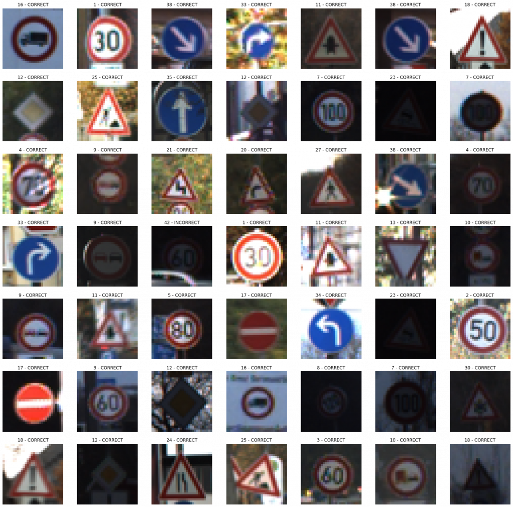
Voila! The model managed to achieve an accuracy of 96.37% on the completely unseen dataset. Let us see how it performs on the images captured from Google Street View.
evaluate_validation(model = conv_model_v11, no_of_images = 32, rows = 6, columns = 6, type = 'sv')1/1 [==============================] - 0s 1ms/step - loss: 0.0781 - accuracy: 0.9688
######################
STREETVIEW TEST Accuracy: 96.88%
######################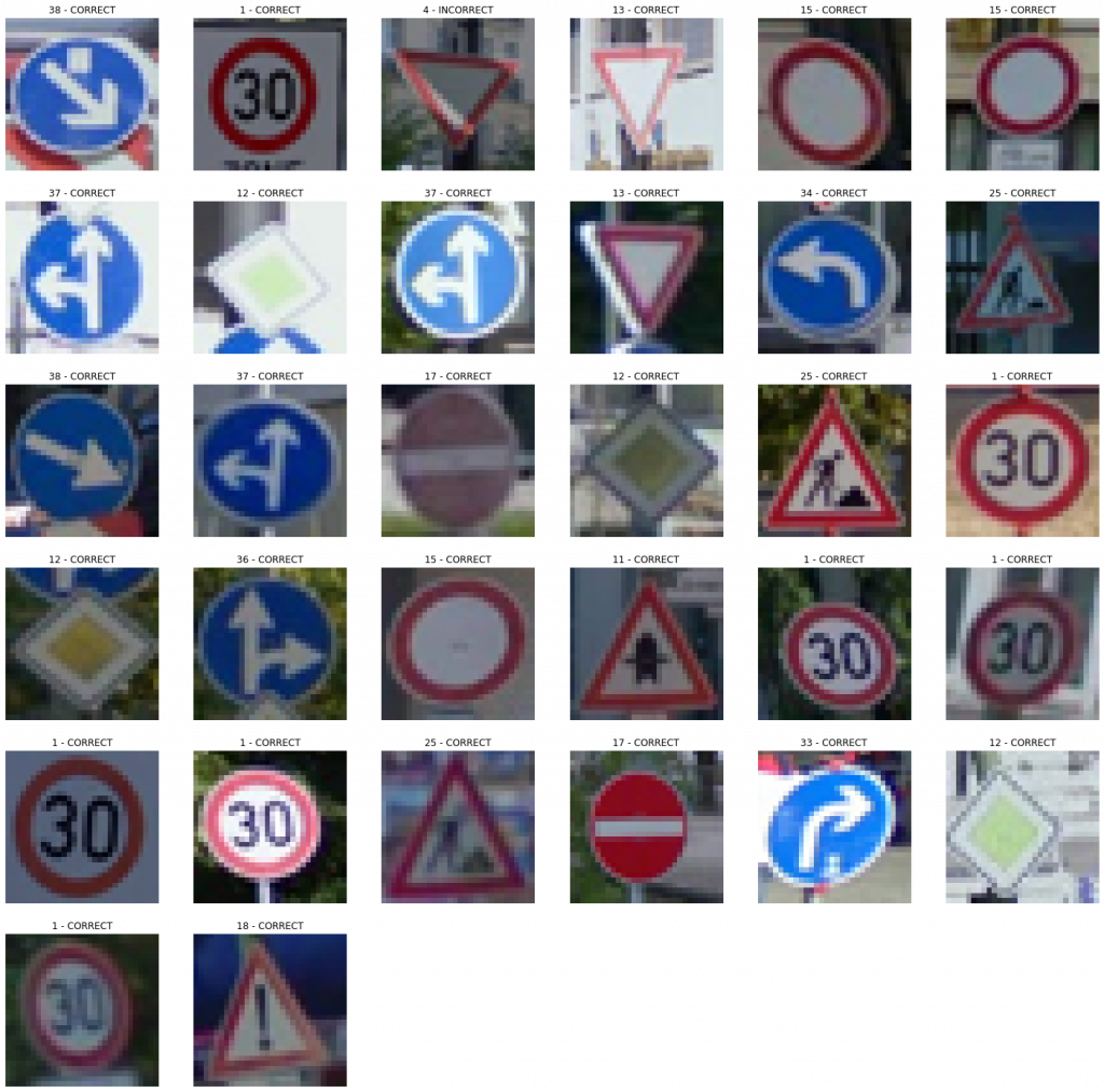
Again, it showed a similar accuracy for a completely unseen dataset. With a little bit of tweaking and troubleshooting, we should be able to improve the performances. But, let us focus on the enhancements on another day. For the moment, we are happy with the output produced by our model.
Do It Yourself!
Here, we will briefly explain how we build a simple, yet effective web application for testing the algorithm on the go. I think that the development of a web app might be beneficial because it showcases our capability to provide an end-to-end solution since we focus on the deployment process as well.
In the previous sections, we demonstrated how you can build a deep learning models from scratch, and test them against different datasets to measure the respective performances. However, we used the Jupyter Notebook interface to handle our coding experiments. We understand the difficulties posed by such an approach if you are a less tech-savvy person. Thus, we hereby present you a handy web application, where the trained models can be utilized by YOURSELF to experience how the models output results.
The application can be reached by visiting the following link, where the necessary instructions have been given for you to easily classify the traffic signs, YOURSELF! Enjoy!
Traffic Sign Recognizer | Do It Yourself!
Feature Additions
Detection of Unknown Images (From 12-07-2021 to 16-07-2021)
After the development of the web application, we realized that the application does not perform up to the expectations when it is presented with an image which does not consist of a trained traffic sign. Since the model had been instructed to strictly output only the designated traffic signs (43), the model was supposed to say that the submitted image belonged to the category of one of the trained traffic signs. This was a problem that we needed to address, and we followed a methodical approach to minimize the issues arising from our problematic approach.
Novelty/Anomaly detection is a research area, where different approaches have been suggested in the literature by the scholars to tackle the problem which we identified. One of the suggested approaches is to include an additional class to the existing list of classes by retraining the model with random images (non-traffic-sign images). Additionally, it is also suggested to create a binary model as a pre-filter which can classify the images by specifying whether the image is a traffic sign or not. For this approach as well, a set of random images are required for training purposes. If we are to follow a different approach, the option is to train a model using an object detection algorithm such as YOLO, and enhance the usability of the web application.
After considering the advantages and disadvantages of the different approaches mentioned above, it was decided to consider one of the first two approaches, because of the comparatively less effort needed to modify our existing model, while meeting our requirement. However, instead of singling out a particular approach, our intention was to implement a solution utilizing both approaches to increase eventual the user experience. As a result, a pre-filter was developed to create a binary classifier which essentially classifies whether an image is a traffic sign or not. After the binary classification, the images are sent through the usual multi-class classifier where the classifier contains an additional class called “Unknown Traffic Sign” to denote images which do not adhere to the characteristics of a trained traffic sign. The following figure illustrates the proposed combined approach.
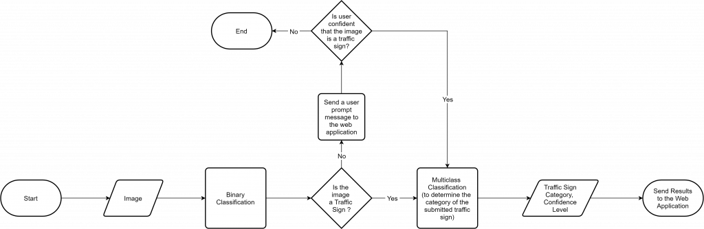
In order to implement the workflow given in the above figure, the following changes were applied.
Adding “Unknown Traffic Sign” to the existing model
- This process increased the number of classes from 43 to 44.
- To achieve this task, 1930 more random images were added from the COCO Dataset to our training distribution, and assigned the new class label (44: Unknown Traffic Sign) accordingly.
- At the same time, 615 images from the COCO Dataset, were added to the Test dataset.
- The same NN architecture that we had used earlier, was utilized with an additional output class, and the model was retrained to achieve a classification accuracy of 99.57% for the validation dataset.
- The model performed well by minimizing the issues that existed with the recognition of non-traffic-signs.
Development of a binary classifier as a pre-filter
- This process entails the development of a binary classifier which classifies whether an image is a traffic sign or not.
- For this purpose, all the images from the GTSRB Traffic Sign dataset (51,839 images) were considered along with 45,670 images from the COCO dataset (non-traffic-signs).
- Necessary splits and preprocessing tasks were applied before the training process.
- Improved the model iteratively (as we had done in the previous version) to create the binary classifier.
- Managed to achieve a validation accuracy of 99.81% and an accuracy of 99.72% for the left-out Test dataset.
Integration
- As elaborated in the above figure, a submitted image first goes through the binary classifier to detect whether the image is a traffic sign or not. If it is detected as a valid traffic sign, the image will be checked by the traffic sign classifier, and a suitable feedback is sent back to the frontend.
- If the submitted image is detected as a non-traffic-sign image, the user is prompted with a message, and the user confirmation is required to proceed further (to force the application to classify the image regardless of its type).
- If the user wishes to proceed, the image is sent
Selecting between PoCs, Prototypes, and MVPs.
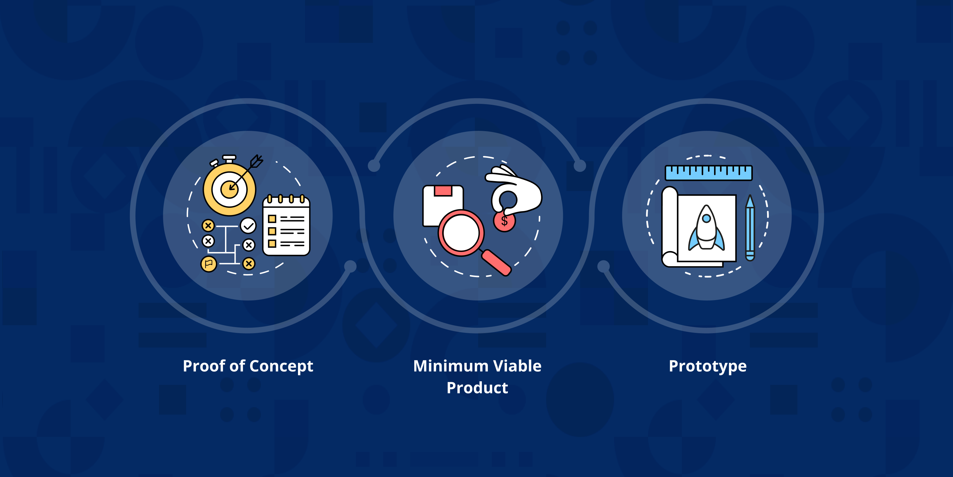
Many companies struggle to choose the aptest technique to validate their concept and choose between POC, Prototypes, and MVP. In our previous context, we discussed the definitions, applications, advantages, and use cases of these elements. You can find the link to the article here and peruse the write-up for a comprehensive understanding.
It is essential to know that it depends on the business idea or the end product and your target audience (B2B, or B2C, B2B2C); and you may need to use PoC, Prototype, MVP or a combination accordingly.
Idea validation using these concepts will ensure that your final product will enable you to achieve its ultimate goal.
A PoC can usually provide a direct response to whether the concept will be viable or not for the target audience. Idea feasibility will be measured here, and with the comeback, you can decide whether to proceed with the existing plan or not. Furthermore, a PoC can help convince your initial pre-seed investors that your concept can be implemented and is technically viable.
On the other hand, MVP enables companies to grasp information about the target user's experience and respond to the core business purpose of the application. The insights received from actual users helps to validate the overall objectives, identify the user pain points, and address the issues over time.
If you want to present how exactly your final product will look like, or manifest the main design elements, prototyping is the best way to give the big picture to the end user. It further helps to run multiple test areas while saving your resources. If you are looking for investors to work on your project, a tested prototype is the best way to demonstrate and pitch your product.
Should PoC, Prototype, and MVP be Throwaway Builds (Minimum Initial Investment)
It is always better to look at PoC and MVP as throwaway codes. If your business idea takes momentum and finds traction, it is vital to build everything from scratch with architecture and design to cope with it for the next 3 to 5 years.
For PoC, think of the least expensive way to implement. Typically, when developing a PoC, factors like product scale, architecture, UI elements are not considered. Instead, the requirement is to check on technical feasibility and customer feedback on your new product idea or a particular feature.
With all things considered, your PoC will be a hardly scalable piece to turn out for something decent. Hence, it is better to consider it as a throwaway build.
In relation to prototyping, it can be either a throwaway or a part of your final user interface, depending on the model type you select. For example, you can use rapid throwaway prototypes to receive user feedback and discard it later. These models are used to validate the system functionalities and requirements. Hence, it needs to be removed as it does not add any advantage to the final UX/UI elements.
For MVP, you may have to build in a way that could cope up with the demand for the next 12 to 18 months (Not a rule of thumb, but empirically proven ). It is common to see startups control the growth without hurting long term plans to build the post MVP version. However, for the long run, it is essential to opt for a complete rewrite ensuring your final product can have flexibility, extensibility and adaptation with upcoming technology and supplementary changes.
A Guide to Choose from Poc, Prototype, and MVP
Exhibiting a decision matrix using a table. - includes questions and scores for users to choose the correct method for their products.
Check out the reference tables at the end of this article.
Decision Matrix
| Parameters | POC | Prototype | MVP |
| Use Case | For Technology/Market/Behavior disruption (completely new idea, so need to prove a concept is viable to build) | To verify user journeys and messaging in a solution are understood by the intended users. Save time and money. Could used to attract seed funding | Get actual users to use your solution to solve the identified problem. Evaluating your solution solves the problem in an acceptable manner. Gather feedback from users to improve upcoming versions of the solution. Aim to the initial target audience response |
| Purpose | To verify technical/market/behavioral assumptions before getting down to development. / To clarify which way to go with the development. Convince internal stakeholders | Make the application usable for its intended users. To assure that the end users could navigate and get the job done using the solution. It is the working model of several aspects of your product. Prototypes help make decisions about product development and reduce the no. of mistakes and waste. | To prove, your solution is effectively solving a problem and it is effective enough for the customer to pay for solution.To get the minimum version of the product to the market |
| Form of implementation | Most rudimentary implementation to prove the relevant disruption is viable to implement | High or Low fidelity Wireframes/UI, users could navigate through different screens but nothing has been implemented | Usable solution by its real user, just to solve the identified problem (nothing more, nothing less) |
| Target audience | Internal users (Decision makers about the project GO/NO GO) | Specifically selected sample of target audience (real users). Should be able to access more than once to verify the prototypes (should be able to involve with iterative process of prototype building) | Sample of target audience. Easily accessible, Give genuine feedback. Test the product with a pre-selected potential customer group |
| Cost | Less budget and is ideal to collect internal funding. Might have to invest on new tools and accessories. | Much less cost to build the prototype compared to PoC or MVP. More time/resources spent here saves time/resource at the expensive development phase | No compromise on quality as the end product would be used by real users. Cut the cost by reducing features, not the quality. Well-defined budgets and looks for investment |
| Human Resources | Requires technical experts to develop the basic concept. Could involve tech related R&D | Less technical resources as no coding / development is involved. Need to recruit testers, Iterative design processes | Here you are developing the actual product (at a smaller scale with less features) So needs full technical expertise |
| Risk Evaluation | PoC involves the highest risk or all. But lessen the risk in upcoming phases. | Reduce the risk in terms of user satisfaction in product navigation | Reduce the risk of losing time and resources of the full scale development |
| User Interaction | N/A since is its used internally | Gives an overview to the end user how the end product will look like with basic elements and navigation. Highly interactive with users but without real functionality. | Full user interaction. UI/UX, Key Functions and even feedback from users also a part of interaction |
| Apparent time to create | If you have several options or if you uncertain about the feasibility of the concept | When you are confident about your idea and needs to start and test the design process | When you are positive about the idea and the design, and ready to launch it to the market |
| When to Show the investors | Pre-seed / Seed | Pre-seed / Seed | Pre-seed, Seed, rarely for Round A |
| Cashflow | Negative (expenses only) | Could leads to Positive cash flows from Investors (Seed level) | Should lead to Positive cash flows from service revenues & Investors |
| Extended use | Can be used to develop MVP | Output can be used to develop the solution. No waste. If the prototype consist of UI design, it could be used for the development | Can be expanded and used for the full version of the product. You may have to throw away the code (Do not hesitate to do so) |
| What you should not do? | Invest time/resources to make the PoC usable to others.Implement things that have been already proven | Use placeholder content or graphics. Train/Assist testers. Test how UI/UX work on real environment | Compromise on quality Implement extra/supplementary features |
| Outsource or in-house work | At this stage, you are working on an idea to check out its possibilities of turning it into reality. Hence, it is ideal to do in-house to ensure that your concept would not be revealed to third parties /competitors. | Prototypes can be fully outsourced as they will be exposed to the public for test-run purposes. | MVP can be done internally or with the contribution of a third party. A mixed team is preferred here to build up the product. Here, the expertise (outsource party) can help with the best techniques while the in-house team is conscious of the progress/development plan. |
Final Take Away
Building a solid foundation is essential to deliver a successful software product. Your PoC, prototypes, and MVP will be your foundation for the process, with actual feedback. They will help you to iterate the product process and enhance the features to meet the user requirements or the ‘real-needs’.
However, software product development is not limited to paying attention only to the initial process but is involved with many crucial steps that need to be considered throughout the proceeding. With that note, the next phase of the development process will be discussed in future articles.
PoCs, MVPs, Prototypes & Throw Away Codebases for Software Product Development
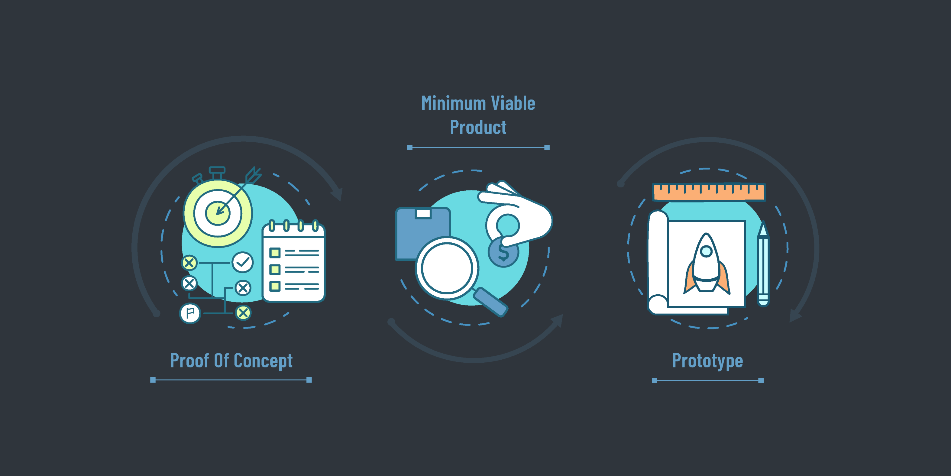
The development of a successful software product requires excellent preparation with a series of steps. Brainstorming, planning, incorporating ideas, designing, QA are a few actions that are involved with the proceeding of product development. Each step helps to validate the stability and the effectiveness of the final product, and hence it is crucial to give equal attention every step of the way.
This is the second of our series of articles where we look into the basic elements that every expertise considers before developing a comprehensive software product. If you would like to keep up from inception, check our first article using the link below.
Link to our first article – The Essential Guide to Software Product Development.
If you are involved in a startup that is based on a new software product, these articles can help you understand the basics of how to go about it in the most economical and methodical way.
Disclaimer
This is based on 20+ years of experience in software product development. After seeing projects succeed, fail, survive, happy clients, angry clients etc. Encountering a mix of positive and negative things has helped this article to chip in a balanced view. It will further assist to learn how to succeed or fail with minimum damages or minimize disasters.
Significance of Software Development for Businesses
Software products have become one of the crucial needs to enhance and upscale any business. Automation of processes through software development helps to cut downtime and manual techniques for a smooth operation.
Streamline of internal functions, improved client experiences, feature-rich additions to the market are some top-notch features of software products that have made it super consumer effective while growing its popularity in every industry.
Problem Analysis
When you boil it all down, you will notice that the initial step of software development is identifying the problem. In other words, the need for a software product comes with addressing a particular issue.
Identifying and addressing the problem will ensure that you have developed the right solution as a software product. However, it is also essential to reckon that the problem and the requirements can be transitory and are likely to change over time.
Looking into the end-users or the target market is another critical point here. While collecting brick by brick for the development process, it is essential to pick out where your final product is going to fall. This could be Business-to-Business (B2B), Business-to-consumer (B2C), Business-to-Business-to-Consumer (B2B2C), or an internal software product development.
Once you have identified the problem and where the final product falls, take notes and put it out in a writing document to present for a group of people or your team. This allows you to receive multiple perspectives and dig deeper to understand the root causes that affect and manifest the main problem.
Pinpointing the primary problem, connecting the contributing factors, identifying the affected people (Eg, project sponsor, customer, user, management), defying the scope of the solution, and recognizing the solution constraints helps to analyze the problem, understand the affected areas and address them accordingly.
Idea Validation
The ultimate goal of idea validation is gathering evidence that your project will end with a paying customer or increase efficiency (to save time or cost). It helps to see the viability of your concept and how it will work in the real world.
Idea validation helps to reduce risks, speed up delivery and minimize costs. Below are a few questions to analyze the demand for your idea or to determine what the final product will achieve.
- Are you targeting the right audience with the correct problems?
- Can the final product help customers/users get their jobs done?
- How often do they need to use the product?
- Can your app solve a problem in a new way? Or is their innovation involved?
Setting up measurable and clear objectives is essential to determine how the idea will validate in the real world. In addition, formulating a hypothesis, developing a value proposition further enables you to get a clear answer.
PoC, Prototype, and MVP
A substantial part of idea validation is covered by following three main ways; use of a Proof of Concept (POC), Prototypes, or a Minimum Viable Product (MVP).
To make it more comprehensible, check out these working definitions for PoC, Prototype, and MVP.
PoC- Works in a controlled environment with a set of preconditions. Typically, a PoC is operated by the technical team and cannot be used by the outside world. However, PoC helps to demonstrate the core challenges or the processes for a particular problem can be addressed using the solution proposed.
Prototype- Gives a clear picture of the design and the user journeys of the application to make sure end-users could use the application conveniently. Users can mainly see the UI/UX aspects here but not the internal functionality.
MVP – A segment of the target audience will use MVP to solve a real-world problem. An MVP is bound with limitations and may not have many features. But the core functionality can be used to benefit from the system.
Depending on the situation, software companies use PoC, Prototypes, MVP or a combination to validate and receive feedback for the final solution.
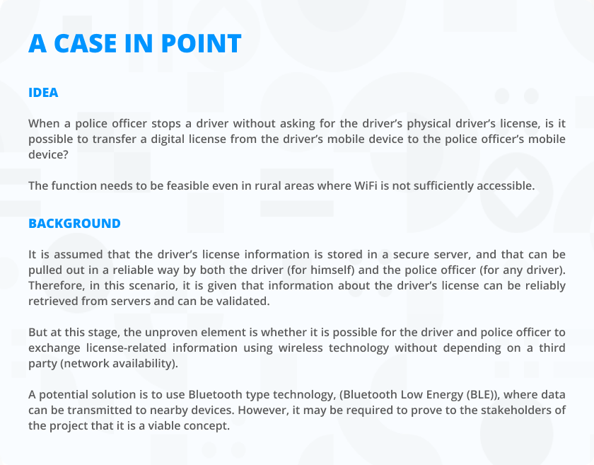
Proof Of Concept (POC)
A PoC helps to pursue ideas before approving them for further testing. It helps to identify the feasibility of the concept and identify potential issues that may affect the final product’s success. Using a PoC, you can determine whether the product can feasibly develop to solve the problem you are trying to solve.
For the most part, a PoC is developed internally in a controlled environment and cannot be assembled or changed. It is a skeleton of the final product with minimal features to test out and distinguish how it will work in the real world.
Given below are a few advantages of developing a PoC during software development.
- It helps to choose the most appropriate technology for the development process.
- Simplify and improve the software functionality
- Receiving valuable feedback before building the actual product
- Potential to get onboard clients before official product release
- Avoid costly mistakes
- Increases the chances of commercial success
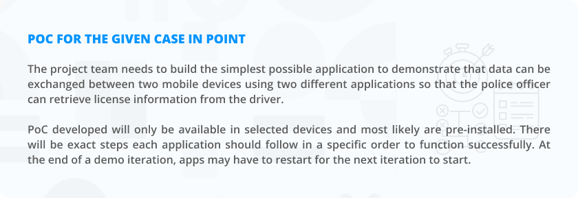
Prototyping
A Prototype is an iterative process that is used to ascertain the UI/UX aspect and visualize your product to validate the user journeys. It will demonstrate the critical design elements and the user flows using wireframes and storyboards. It helps define the features that need to be included and makes up a model to expose the errors in studying and designing.
Typically, there are four prototyping models, namely, Rapid, Evolutionary, Incremental, and Extreme. In most cases, following a PoC, a prototype is used to obtain further details of your final product and to see how it looks and users would use the features in the end.
Identifying customer needs, enhancing product workflow with better understanding, identifying design and related mistakes are a few advantages of prototyping in your early product development process.
Most importantly, you can also use it as an opportunity to reach the users at an early stage and get their feedback before putting your product into the market.
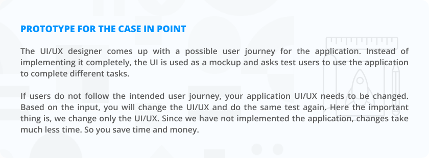
Credential App


Reader App


Link to walkthrough a sample prototype
Prototype of Credential App – Live demo
Prototype of Reader App – Live demo
Minimum Viable Product (MVP)
Typically, before releasing a full-fledged product, an MVP is used to collect feedback from early customers. The responses from the real world help developers to work on the versions and improve the product accordingly.
An MVP consists of the core features and the minimalist design that deploys the final product. The basic infrastructure is developed using the least possible expenditures and has certain limitations. Positive and negative feedback received from MVP help validate the idea of the final product and see the potentiality of its success. It can also be used to solve an existing problem or could be used to improve the efficiency (cut down of effort taken, time taken, or cost involved) of a task.
MVP introduces efficiency to a selected task (core problem your application solve), and there could be many other auxiliary features that could improve the efficiency of the same job. But with the MVP mindset, you will not try to include those complementary features in the solution you provide at the MVP stage. So, again, that’s why we call it MVP. Solve the intended problem, but nothing more, nothing less.
There are different types of MVP concepts that can be used based on the purpose. Software prototypes, product designs, concierge, landing pages, piecemeal, demo videos, and wizard of Oz are some of the main ways the MVP concept is used. Dropbox, Amazon, Airbnb, and Facebook are a few well-known examples that started with the MVP technique.
Below are the key advantages of using MVP.
⦁ Avoid lengthy unnecessary work
⦁ Gain insights on product viability and usability
⦁ Saves project time and money
⦁ It gives clarity around the final product idea
⦁ Analyze market demand

When you disregard all non-essential features, that brings the time to market your product less and cost to develop your product less. These are the pillars of lean product development.
Choosing between POCs, Prototypes, and MVPS could be crucial to find the aptest solution for your business proposition. Furthermore, after considering all these essentials, you could decide on selecting them as throwaway codebase elements or not. Hence, our preceding context will discuss the guidelines and the necessities to choose between these elements.
We want to thank Chalinda Abeykoon for being a part of this effort and adding value to this article by sharing his insights and experience.
Stay tuned for our next article.
How Fidenz, a Software Product Development company helped Iper to scale its business by leaps and bounds


The Client
Iper Direkte AS is a Norwegian-based marketing company that provides up-to-date marketing-related information about consumers and businesses to interested parties. The type of information they provide includes personal, property, vehicle, and more. Iper uses a powerful matching system to identify and extract the above information to be used by its clients.
 Iper’s Business Challenge
Until 2014, Iper didn’t have a fully automated system to run its business workflow smoothly. They faced difficulties in scaling their business due to the following reasons.
- Data were collected and stored locally in on-premise infrastructure.
- Data lists were created manually by Iper’s internal staff.
- Data was shared using simple file sharing methods like FTP.
- Billing and accounting were done manually.
These issues were a major stumbling block in the further growth of their business. It is during this time that Iper felt the strong need for a robust digital platform through which they can fulfill their customers’ needs faster and better. They wanted a state-of-the-art platform that can deliver on an autopilot system independent of its number of employees.
Iper tried to automate their business process with the help of some local and nearshore software development teams but all in vain, because they failed to bring the desired results. Iper realized that building such an advanced system in Norway, one of the most expensive labor markets was not feasible in an ROI-friendly manner.
 The Solution
While searching for a trustworthy partner who could build their software platform, they heard about the small island nation, Sri Lanka, where IT services outsourcing is booming. Partnering with an IT service provider in Sri Lanka, a country located 8,000 km away from home, is like exploring uncharted territory. After careful thinking, they overcame this mental block. They took a courageous decision, a calculated risk; they finally decided to identify the best software development service company for them in Sri Lanka to be their ideal partner and landed in Sri Lanka.
In Sri Lanka, many companies came forward to offer their services but what Iper was looking for was someone with that ‘special edge’ with whom they can build a long-term relationship and also someone who can show genuine care and interest to grow with Iper.
After a series of meetings with us and a few technical evaluations, they discovered that we could deliver exactly what they needed, and above all, they spotted that spark within us to excel at what we do and thus Fidenz was chosen by Iper as their most promising partner to provide them the necessary software solutions.
 What We Delivered
After initial brainstorming,we decided on the exact platform that Iper needed.With extensive research and review, we came up with the PoC for the platform. The PoC proved to be successful and it was agreed upon to deliver the project as a fixed scope, at a fixed timeline and fixed cost.
Identifying the MVP (Minimum Viable Product)
We identified the MVP and made sure that the features we chose for our MVP could be completed within a time frame of 3 months.
As MVP features we decided to add the features most used by current Iper clients and features that could be simple enough to be used by Iper clients with minimum training.
Our careful selection of features for the platform enabled Iper to evaluate the effectiveness of their digital platform with minimum cost and time. Not only that; Iper, during this time, had the opportunity to evaluate Fidenz in all areas and aspects. At the same time, the Fidenz team felt passionate about the project and realized how easy it was to work with Iper. Altogether, it was a harmonious relationship in which both had developed a deeper heartfelt connection towards each other.
Our Development Process
Once Iper was happy with the MVP, we started our development process. We started our development on the Microsoft Stack but gradually integrated open source elements. We introduced ‘Elasticsearch’ for free text search, which is a highly scalable open-source, full-text search and indexing engine. It allowed us to store, search, and analyze large volumes of data in near real time thus giving extraordinary performance to the system. Elasticsearch was the first open source element we used in Iper platform and this infused an interest in Iper to use more and more open source tools whenever possible.
Over time, we have developed many features and improved the platform significantly. Currently, we are working on introducing micro services, aiming to save costs by utilizing resources on demand (pay only for what we use).
We introduced new technologies to minimize the cost on a mid to long term basis. As a result,ROI increased over time and Iper managed to invest more and more on platform improvements.
Further we ensured that the entire system could grow continuously both vertically and horizontally. Horizontal growth allows more and more features (connect more data sources to the data warehouse and make more data available via Iper APIs) to be added to the core framework while vertical growth allows enhancements to the framework itself in terms of scalability, reliability and usability.
Documentation
Our product documentation includes information for managers, end-users and developers on how to administer the system, how to use the system and how to integrate external systems with Iper platform respectively.Technical documentation generated for Iper includes information on requirements, architecture & design, infrastructure, and all other aspects of the platform development process.
Using reliable tools such as Confluence, BitBucket and JIRA in our product development process has given us the opportunity to produce robust and maintainable platforms. Confluence is used to organise and store complete knowledge about the platform in a single place. BitBucket is our version controlling tool for source code and JIRA is used to capture requirements and issues. We integrated all the three tools comprehensively together to take a snapshot of the project at its current state and at any point in time in the past.
Developing a platform that could be managed by minimum resources was of paramount importance for the client right from the very first day. Currently, any new developments, feature enhancements, technical support, and all other aspects are managed by a team of two dedicated engineers. The brilliant design and architecture and detailed documentation have paved the way to achieve this objective. That’s why we believe that what we have developed for Iper is a true engineering masterpiece.
 Conclusion
In a nutshell, Fidenz succeeded in winning Iper’s heart as one of the most trusted software development service companies in Sri Lanka who helped them to scale their business manifold in a cost and time-effective manner.
How Iper felt about Fidenz in their own words
“We still remember how uncertain we were when we left Gardermoen airport to meet with Sri Lankan companies back in 2014. But after 6 years when we look back now, it is one of the trips that changed a lot for Iper. Partnership with Fidenz opened doors for us to offer technically advanced and state-of-the-art solutions to our clients around the world. The Fidenz team has been the trusted partner for us all these years and how they collaborated with us to improve our core business platform over time is remarkable. They always understood our business needs and shared their thoughts with us on how to improve our offerings using technology. Their ability to look at our business from different angles made our platform affordable to improve and maintain yet adaptable to face the unknown future.”
The Essential Guide to Software Product Development

Software product development is an avenue with immense potential across a range of industries. However, with these ample software product development opportunities comes concerns that businesses might not think about or fully understand before developing their software.
There are common issues, such as increasing customer demands and limited resources, as well as issues that are specific to your business that can be solved using software products or platforms.
These software products and platforms can help your business succeed in two primary ways. First, they can help you expand your business through various means such as improved marketing and outreach or even analysing data for new markets your business could fit. Second, they can help increase your business’ efficiency leading to a larger profit margin allowing you to direct your revenue towards more growth.
So, as the first step to our series of articles, we will guide software product development and introduce the opportunities that await your business within this field.
Disclaimer
The information discussed in this article bases its report on 20+ years of experience in software product development. This assessment comes from two decades of watching projects succeed, fail, survive, produce happy clients, and angry clients.
Therefore, this information will provide you with a mix of positive and negative aspects of software product development. This overview is purposefully inclusive, providing a balanced view of succeeding or failing within this endeavor with minimum damage or minimized disasters.
Why Should You Build a Software Product?
There are many reasons why a business would opt to build a software product. Despite the vast differences in building a software product and most traditional retail products, the reasons for making your software product are similar to creating any other product or business:
- You have an idea for a new project: If you have an idea for software that solves a problem more efficiently, you could have an entirely new project idea, with the core of the project being increasing the efficiency of your business.
- You have an idea for creating a support service: If you have an idea that will help save time, money and ultimately leads to better profitability within your field, or even within another area, that could be a seed to build a software product around that.
- You need software to suit your unique needs: Most of the time, people create software and other inventions or upgrades based on their needs. Sometimes, out of the box products do not suit your unique needs. While it still might be cheaper to create a workaround to manage this issue with the out of the box option, sometimes that is not possible. Therefore, it is worth the time, money, and effort to save yourself (and others) these headaches in the long run.
How to Start a Software Product Development Project?
Starting a software product development project is not an easy feat, regardless of the tools and options you have at your disposal. However, it certainly does help to know that you do have options. You do not need to start from scratch as there are primary resources available for nearly any kind of software you intend to develop.
Here is what the technological world has to offer as cornerstone options to kick off your software product development:
PoC

Proof of Concepts (PoC) help you prove that your software will work in the real world. This demo system simulates real-world stressors on a concept to ensure the real version of the conceptualized design will perform as designed.
This environment test helps prove that the concept will work, before the time, money, and energy gets invested in creating the real deal.
MVP

Minimum Viable Product (MVP) is a resource that decides whether your software product can actually solve the problem you intend to solve. MVPs are especially important with software development because it tests the idea of change versus need. MVP will determine whether your software is solving an actual problem your end users are experiencing and if they’re willing to pay for that solution.
Throw away vs. Built to scale
Throw away and Built to scale are two fairly self-explanatory methods to start your software product development.
Throw Away Software
Utilizing the throw away approach to starting your software product development means you built either a PoC or MVP you know cannot be turned into a commercial product. It’s typically built with minimal time and resources purely to test your idea. Once you’ve tested your idea, you’ll need to completely scrap all previous development and rebuild the software product from the ground up. This allows you to confirm you have a strong idea for a software product without wasting time or resources.
Built to Scale Software
Much like the name suggests, built to scale software is a product and resource that should grow with your business needs.
While a throw-away software build is a bandage, build to scale software is a skin graft. There are many opportunities within the build to scale software development because it intends to evolve and thrive even though the upfront costs are higher.
Should You Use a Throw Away Build or Scaling Build for Your PoC or MVP?
A lot of throw-away builds are specifically for PoC or MVP. These builds require minimal time and investment, as they are only demoing your concept. If your idea for your software product is unique or completely new to its target market, then building a throw-away product allows you to test your idea with minimal resources.
However, most software product development projects should start with scaling in mind. Built to scale software does take a moderate initial investment but pays off if you continue because you have already laid the groundwork for the actual product, instead of just a demo. If the solution you are building revolves around a proven business model, then using a scaling build will allow you to grow it faster as you’ll already have a usable code-base.
Decide Your Tech Stack

Besides having options for creating concept designs, technology advancements also offer you different options for your preferred tech stack.
Using similar Open Source projects Vs. Built from scratch.
The foundation of your software will come from two broad options:
Open Source Projects: Open source projects are created by other software developers or coders who have shared their work with the general public. If you can find an open-source project to help frame your software development code, you can cut out a lot of initial time, money, and resources.
Pros of Similar Open Source Projects:
- Low initial costs
- Highly reliable (not every project, but you could easily figure out the quality)
- You still have the flexibility to make it yours.
Cons of Similar Open Source Projects:
- There are potentially long-term costs needed to keep it running.
- Would not match with your exact requirements
- It could pose serious security risks.
Building from Scratch: Exactly how it sounds, building from scratch creates an entirely new code without any business specific foundation to start you off.
Native vs. Cross-Platform
Building your software product as a Native or Cross-Platform solution will be a decision that you need to make if you are creating an app for mobile devices. Thankfully, the basic concept of native and hybrid software development is relatively easy to understand.
Native: Native app design is when everything for that app is designed specifically for one operating system (iOS or Android.) While you can create an app for each platform, you will have to deal with multiple code bases instead of one.
Cross-Platform: This option of app development ensures one code base produces an app for each operating system.
Remote vs. In-House Team

Remote work is becoming more commonplace, but there is still a notable divide on whether you should hire a remote team or keep your development team in-house.
Remote Team
Hiring a remote team in this context means you are outsourcing your software development team. Therefore, remote resources are all contractors who don’t work for your company, even though they can be bound to secrecy and nondisclosure, depending on your agreement’s arrangements.
Pros of a Remote Team:
- Low cost (usually one third compared to inhouse)
- Minimum commitment (you could terminate your contract easily)
- Quick kick-off
- Fast turnaround
- Diverse tech skills (on demand)
Cons of a Remote Team:
- Their commitment to you can also be minimal.
- More of a security threat
- Could just disappear without finishing the job
In-House Team
Creating an in-house team is an investment. Chances are, if you are developing an in-house team, you are expecting to be in it with the same people for the long haul.
Pros of an Inhouse Team:
- Easy Communication
- You get to know their work habits.
- You have more control over their loyalties.
Cons of an Inhouse Team:
- High cost due to:
- Full-time (or Part-Time) Salaries
- Other Benefits
- Difficult to find skilled resources
- Takes a long time to build an effective team.
Make Your Software Future Proof
Of course, no one knows what the future holds but by making an effort to future proof your software product before you spend too much money and time developing it. Here is the best way to future proof your software development:
- Validate the idea with minimum cost
- Your project may or may not succeed but invest time to think about both scenarios before kicking off the project.
Where Can I Find More Information on Software Product Development?
This essential guide to software product development provides all of the basics you need to kick-start your software product development efforts. Of course, there are an extensive set of details to each section of this guide that will help you develop your software product in the most efficient and effective way. So, we will be creating future guides to each specific aspect of this overall guide you can utilize for a comprehensive look into software product development and how it can help your business thrive.
Link to the next blog – PoCs, MVPs & Throw Away Codebases for Software Product Development
Agile Transformation: How Agile Software Development Has Gone Mainstream
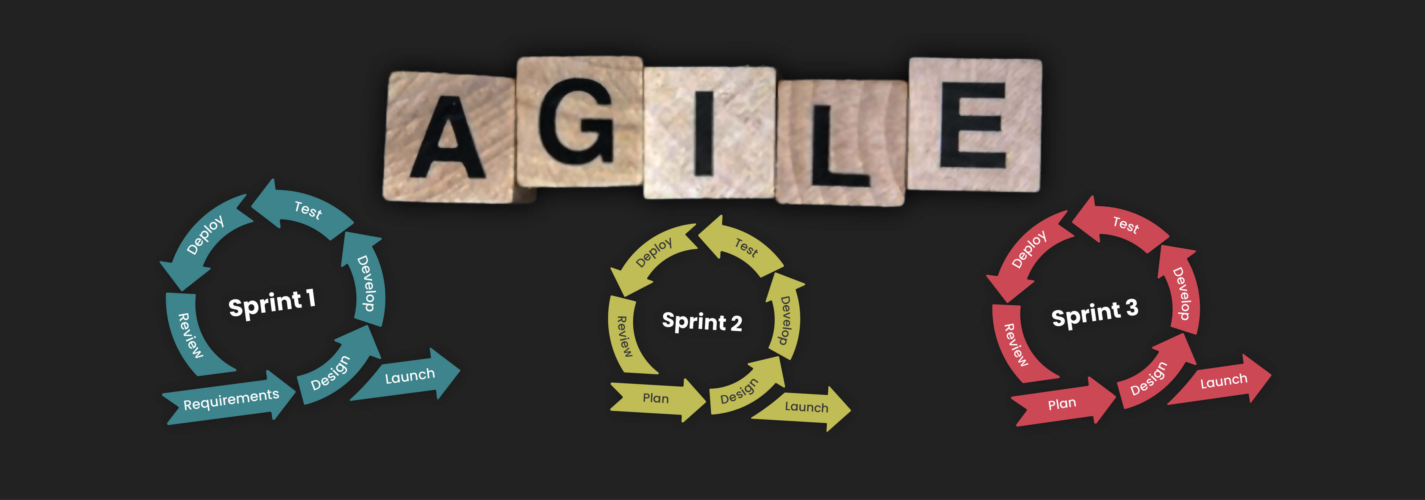
In software development methodology, with the thought of “How to make an idea into a reality,” the agile method is the first thing that comes to mind to step up into the process. In simple terms, agile is a set of values and principles that teams can use to make decisions on developing software.
Evolutionary project management and software development methods can be traced back to 1957 where heavyweight methods were used in the development process. Lightweight software development methods started to evolve in the 1990s with different executions.
The traditional waterfall or the incubate method takes a lot of time and work and is often described by critics as a micro-managed and overly regulated methodology. The collection was inclusive of 17 software development methods where the developers met in 2001 and published the manifesto of Agile Software Development.
Overview of Agile
With the publication of the manifesto for agile software development, four values were outlined by the Agile alliance. These values enabled a faster process, excellent customer collaboration, adapt and revamp planning and put people before processes. The values are:
- Individuals and interactions over processes and tools
- Working software over comprehensive documentation
- Customer collaboration over contract negotiation
- Responding to change over following a plan
Furthermore, it was finalized with 12 development principles. These fundamentals help user involvement and a cooperative approach where stakeholders can monitor and examine the progress of their products. It further helps in identifying issues during the development process and gives assurance of achieving satisfying expectations. The 12 agile software development principles are;
- Customer satisfaction with prompt delivery of valuable software.
- Welcome changing requirements, even in late development.
- Deliver working software frequently in shorter springs
- Close engagement and collaboration between business people and developers
- Projects are built around trusted motivated individuals
- A face-to-face conversation is considered as the best form of communication
- Working software is considered as the initial measurement tool of the progress
- Sustainable development is used to maintain a constant pace
- Constant attentiveness to technical excellence and designing
- Use of simplicity and maximizing the amount of work not done is required
- Use of finest architectures, requirements, and designer ideas.
- Regular effectiveness and adaptability of the team for adjustments.
How Agile Has Gone Mainstream
The methodologies and applications of agile have led to the mainstream in software development with proven results in making efficient and effective products. The diversification and constant changes in technology have raised the need for flexibility and adaptability of software to meet future changes. With agile, products were engineered and developed in a way that they are nimble enough to adjust to the changes and the businesses.
The global competition in every industry to develop the best user-friendly and feasible product keeps rising with numerous attempts from all corners of the world to deliver the most refined technology solutions. Hence, business owners often prefer a method that can create a more durable, flexible product to beat competitors. The practices used in agile methodology come in handy here to deliver a top-notch solution.
With the Agile method, practices like MVP are used to get faster test runs and feedback from users before developing the complete solution. This helps to receive an assurance on the strategies used and to receive an idea of the success rate of the ultimate expectation to build up the business value.
The stakeholder engagement before, between, and after each sprint results in higher collaboration and helps to deeply engage in the project, which eventually results in delivering a high-quality product. It further helps in transparency where clients can be involved in prioritizing features and other changes with the right guidance and understanding in each review session.
The agile method of software development also helps in improving quality by breaking down its units where the team can focus and concentrate more on each section with testing and reviews. It also helps in finding defects easily and quickly and figuring out the mismatches that need to be altered accordingly.
The powerful tool of agile consisting of components such as project planning, roadmap creations, sprint planning, sprint reviews, and retrospective helps every participant to enhance the product quality in terms of control, flexibility, adaptability, etc. The testing methods help in developing a product speedily and cost-efficiently while focusing more precisely on the final goal. It helps to overcome pitfalls like scope creep and waive off the unnecessary costs while engineering the product.
Practicing these methodologies helps the development team to work collaboratively with higher transparency to deliver a product with a higher success rate. It further aids in developing software that is nimble enough to adjust to future changes and requirements in the business.
It is essential to find a team that follows these practices and principles of agile correctly during a software development process to deliver a high-quality, superior product. At Fidenz, we have a proven record of building successful products with the right strategies and implementations. If you are looking for a software solution to upscale your business, contact us to receive the best consultation on product development with agile methodologies. Our team can provide you with robust software solutions that can serve your organizational goals and adapt to future changes along the way.
Explore a Few Real Uses of Blockchain Technology

The term blockchain is often misinterpreted as a single-use for cryptocurrency and bitcoin transactions. However, the application has not been limited to these two and has numerous other uses in diverse sectors. This article will look into a few real uses of blockchain and how it can revolutionize technology benefiting different industries to enhance their work.
An Overview Of The Blockchain Technology
A blockchain is a type of a database that collects information or stores transactional records in groups or in other words “blocks”. When these storage capacities fill, they are chained into the previously filled block, forming a “chain”. With its most prominent usage in cryptocurrencies, the storage is often called a digital ledger. This information stored here is highly secured, and each transaction is authorized by a digital signature authenticating the transactions. The following characteristics of blockchain technology have made it immensely popular over time, diversifying and multiplying its uses.
Decentralized system : Unlike the conventional methods, blockchain transaction takes place in mutual
agreement of users.
High Security : The digital signature feature has made fraud transactions and data corruption
impossible.
Automation Capability: The technology is programmable and can generate automatic system actions, events,
and payments.
Uses of Blockchain Technology In Different Industries
Applications in Financial Services
Embracing the blockchain industry in the financial sector has enabled us to lower the expensive mistakes that come with human errors, operational risks and streamline each process. The blockchain applications in financial trade allow recordkeeping, onboarding, security, privacy, data management, and trade processing secured and efficient. Features such as digital document authentication enable real-time verifications and collation of user activities. The tracking and enforcement of regulatory controls facilitate the collateralization of assets. Digitizing the lifecycle of finance with blockchain applications can enhance the overall security and efficiency of every subsidiary process.
User Identification Process / Digital Identity
The need for companies to comply with Know Your Customer (KYC) policies has become crucial over time. The guidelines enable financial sectors to manage risks prudently and prevent activities like money laundering. In order to meet user identification standards, blockchain can facilitate a standardized network of identification information. The data can be stored and accessed securely and validated in record time. The digital identity applications through blockchain can be used in many sectors, including finance, health, education, travel, etc.
Blockchain-Based Cloud Storage
Cloud storages have numerous advantages, which include usability, easy access, automation, cost-efficiency, synchronization, convenience, etc. However, some may find cloud computing problematic with the risk of cyber-attacks. Integrating cloud storage with blockchain can carry off the problem with its extremely secured segments. The data of blockchain-based cloud storage is divided into many encrypted segments and are interlinked through a hashing function. The decentralized locations and security provisions assure reliable and robust security against hackers. Further, they do not hold the data on a node and hence help owners to retain their privacy.
Smart Contracts
With an objective of reduced intermediates, fraud losses, enforcement costs, arbitrations and other accidental exceptions, smart contracts are used to execute and control agreements. These contracts include legally relevant events and actions with the terms between the buyer and seller written into lines of code. The smart contracts are available as a computer program or a transaction protocol, and the codes control the execution while making traceable, transparent, and irreversible transactions. The self-executing contracts permit trusted contactors and transactions even among anonymous parties without the requirement of a centrally authorized legal system.
Blockchain For Logistics
Blockchain solutions for the logistics industry can provide extra transparency and clarity to all of its stakeholders. The applications can allow documentation and recording in a digital platform, making it incorruptible. The important paperwork can be stored in the form of digital copies and used for updates in the future. It can further track the financial transactions, record them, make POs, custom duties, and other work easy. Record of temperature zone is another key feature of blockchain for cold storage supply chain operations. This helps in improving safety movements and reducing disease spreading. Serial numbers, bar codes, RFID tags, and products are a few hardware tools that can be digitally linked with a blockchain tracking software.
Apart from these, blockchain is used in IoT, voting mechanisms, real estate, royalty tracking, and many other related industries. The improved security system using cryptography has enabled blockchain to mark its territory in many sectors.
If you are looking forward to using blockchain in your organization and strengthening your business’s core system, contact us at Fidenz Technologies for ultimate solutions. Our team of professionals is happy to help with all your software concerns.