A CNN Approach for Recognizing Traffic Signs
Introduction
Deep Learning is an interesting and a unique field of study that has attracted the worldwide attention over the past few years at a rapid pace. The rate at which the digitalized systems have been generating data for over a decade, has become one of the major reasons for creating an abundance of data. As a result, the availability of data provided a brand new perspective for the researchers to look at Artificial Intelligence and its branches, in a different way. Additionally, the gradual enhancement of hardware resources resulted in offering much improved computational resources for the deep learning researchers to make use of data efficiently. Therefore, the combination of data and modern computational resources, was able to create a platform for the researchers to thrive on, and the result is a highly motivated deep learning community that continues to contribute towards the growth of deep learning using novel approaches. Computer vision is a research area that has benefitted largely from the rise of deep learning, and it is evident from the amount of research studies carried out in computer vision with deep learning.
While there are many specific applications of computer vision, the uses of deep learning in traffic/road related applications, is an interesting application since it directly affects the improvement of vehicular automation. Although the field of vehicular automation is on the verge of reaching greater heights, as evident from Tesla’s Autopilot feature (and similar implementations from other major automobile manufacturers), understanding the fundamentals of deep learning remains an integral part for those who are interested in exploring the capabilities of deep learning. In this article, we focus on bringing you a primer for understanding how the nuts and bolts of deep learning can effectively improve the metrics that measure the success of a specific application that targets traffic signs. Thus, our attempt is to explore the process of developing a traffic sign recognizer using the concepts of deep learning.
We have structured the article in way that allows you to easily move to the desired section with ease. Initially, we explain the Background behind the problem before coming up with an Exploratory Data Analysis for the dataset which we utilized. Afterwards, the Deep Learning Workflow provides a high-level overview of the procedure followed by us, and then we place our emphasis on creating a suitable Input Pipeline for preparing the data to meet the requirements of the Models explained in the subsequent section. Finally, we examine the performance of the developed model, before capping the article off by deploying it as a readymade model which can be tested by yourself using an interactive interface. Sounds interesting, huh?
Background
The Problem
A brief writeup on the actual problem that we are attempting to address. In our context, the broader problem is to check the possibility of recognizing the traffic signs via the concepts of computer vision.
What will straightly come to your mind if you are asked to think of a main road in any part of the world? Obviously, the pedestrians and vehicles should greet your mind as they make the roads busy, thanks to the continuous movements made by them. The clutters of vehicles and pedestrians can certainly lead to unpleasant outcomes, and as a result, standardized road rules have been set up by the authorities to minimize the clutters and to streamline the traffics in a structured manner. Since the drivers and pedestrians are supposed to obey the rules, having assistive signs/lights can definitely help both the drivers and pedestrians to ensure that the road is a safe environment for everyone.
This is where the importance of traffic signs, comes into the frame to act as guidelines for both drivers and pedestrians. While the traffic signs are supposed to be understood by human vision, it is interesting to if the same phenomenon can be emulated using computer vision. In this article, we attempt to address a basic problem, in which we check the possibility of recognizing the traffic signs via the concepts of computer vision.
The Aim (and objectives)
In a broader context, our aim is to develop a recognizer that correctly classifies a given traffic sign image to determine its class, using the concepts of deep learning in computer vision. It is expected to achieve the aim by methodically following the objectives given below.
- Exploring the health of the dataset by performing an Exploratory Data Analysis
- Preprocessing the data for building the input pipeline
- Defining a suitable methodology that iteratively improves the performance of the model.
- Testing the performances on unseen datasets.
- Developing a tool for allowing the user to self-test the capabilities of the developed model.
The Dataset
As we explained in the Introduction section, datasets play a pivotal role in the development of a deep learning based solution. Fortunately, there are freely available datasets for achieving our requirement. Therefore, we used the German Traffic Sign Recognition Benchmark (GTSRB) dataset provided by the Institut für Neuroinformatik. The dataset has been initially provided as a multi-class classification challenge at the International Joint Conference on Neural Networks (IJCNN) 2011.
Exploratory Data Analysis
The Exploratory Data Analysis (EDA) is a common component that provides a representation of the original dataset using descriptive statistical methods with the aid of relevant plots. For more information, refer the following link:
What is Exploratory Data Analysis?
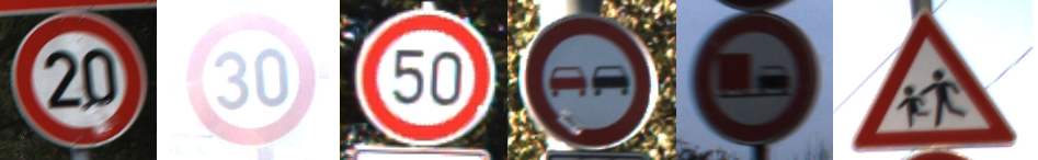
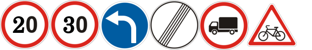
Once we downloaded the ZIP file from the source given above, we came across datasets corresponding to three distinct categories inside the ZIP archive: Train, Test, and Meta. The images related to the Train dataset were stored inside the Train folder where separate sub-folders had been created to organize the Train images under different class labels. In contrast, the images related to the Test dataset were directly inside a folder named Test. The Meta folder was composed of computer-illustrated images to represent each class label and few of the images from all three categories are given below. Additionally, the archive contained three annotated Comma Separated Files (CSV) named Train.csv, Test.csv, and Meta.csv. The composition of each CSV file, is further discussed within this section in the following paragraphs.
Train
Sample Image from the Dataset
Number of Images
In order to explore the number of available images in the Train dataset, the Train.csv file can be analyzed. The Pandas library in Python is a useful tool for dealing with CSV files by including the data into a Dataframe. Based on the results, the dataset contained 39,209 images.
Number of Classes
The dataset consists of images corresponding to 43 classes, numbered sequentially from 0 to 42.
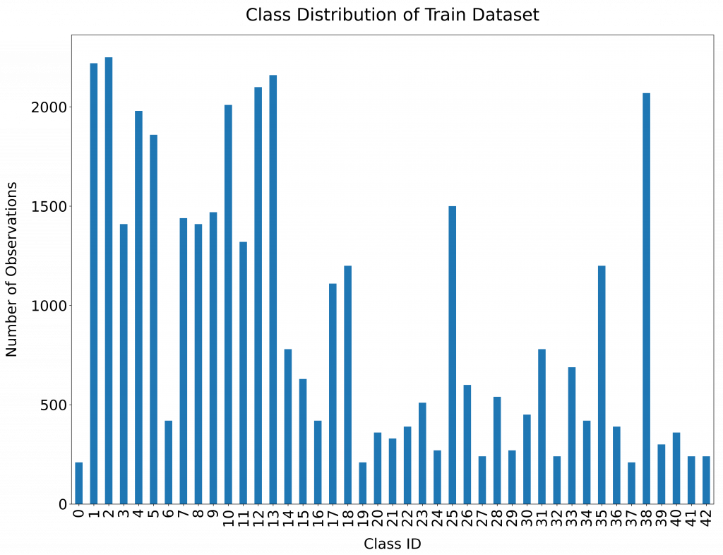
Class Distribution
The following figure represents the class distribution of the Train dataset.
Structure of Data
Altogether, the Train.csv file contains the following list of important fields which can be utilized as per the requirements [Ref: German Traffic Sign Benchmarks ]
- Width: The width of the image in pixels
- Height: The width of the image in pixels
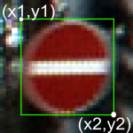
- Roi.X1: The X-coordinate of top-left corner of traffic sign bounding box
- Roi.Y1: The Y-coordinate of top-left corner of traffic sign bounding box
- Roi.X2: The X-coordinate of bottom-right corner of traffic sign bounding box
- Roi.Y2: The Y-coordinate of bottom-right corner of traffic sign bounding box
- ClassId: The actual class label
Test
The annotated file for the Test dataset (Test.csv) also follows a layout similar to the Train.csv.
Sample Images from the Dataset

Number of Images
The Test dataset consists of 12,630 images as per the actual images in the Test folder and as per the annotated Test.csv file.
Number of Classes
As expected, The Test dataset also consists of images corresponding to 43 classes, numbered sequentially from 0 to 42.
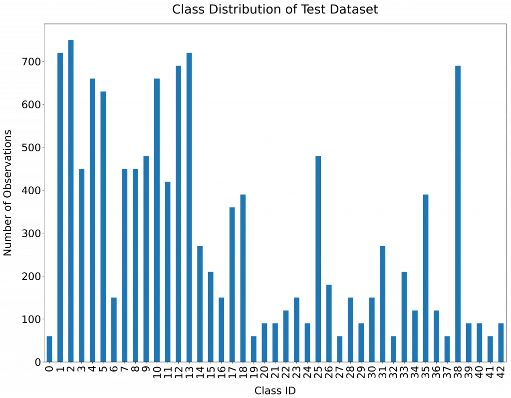
Class Distribution
The following figure represents the class distribution of the Test dataset.
Meta
The Meta Dataset, along with the Meta.csv has been provided as a guideline to represent the actual images and the related Class labels.
The Deep Learning Workflow
Here, we will add a high level diagram for explaining the iterative workflow that we follow throughout the model development/improvement process. The diagram will represent the usual Machine/Deep Learning workflow, with specific customizations to cater the expected outcomes of our case study.
Over the years, the machine learning community has adopted a certain workflow that keeps them in the hunt for the reaching the desired aims and objectives. The following figure depicts the workflow which we usually follow in the process of developing machine/deep learning applications. In reality, deep learning is a highly iterative process that requires the developers to keep experimenting until the target objectives are achieved.
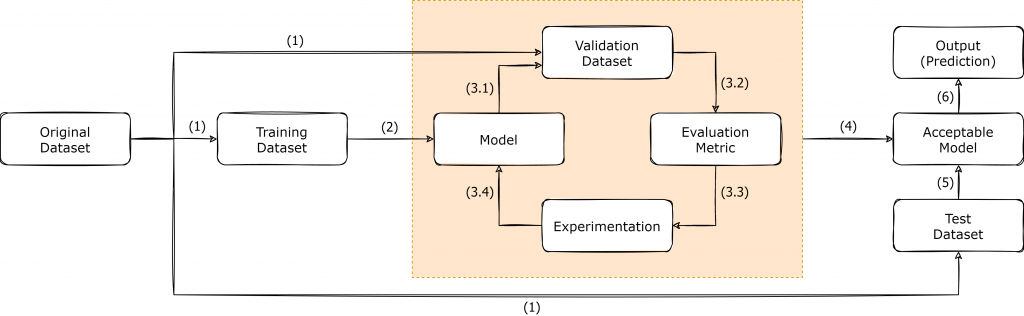
As shown in the above figure, once we have a dataset which is suitable to be applied for a deep learning task, the dataset is usually split into three subsets, known as Training Dataset, Validation Dataset and Test Dataset. The splitting process may vary, depending on the original dataset that you have, and in the context of GTSRB dataset, the authors had provided both the Training Dataset and Test Dataset separately. Since the Validation Dataset is not available in GTSRB dataset, it is up to the developers to decide the best possible way forward for creating a Validation dataset, depending on the application.
Once the Train/Validation/Test split is finalized, the Training Dataset is utilized for training the initial model, as shown in Step (2). The creation of the model initiates the iterative cycle where the model is tested against the Validation dataset to obtain the necessary evaluation metric. Based on the result of the evaluation metric, the developers are supposed to keep on experimenting and form a new model and follow the same cycle, until a model with a viable evaluation metric result is obtained. After the finalization of a model, it is considered as the Acceptable Model [Step (4)]. The Test Dataset consists of real-world data that the model has not previously seen and it provides us the opportunity to Test the created model against real-world data to actually see how it would eventually perform on the production run.
The Input Pipeline
In this section, the focus will be placed on the explaining the preprocessing steps which we followed, before the development of models.
For instance, the process of preparing Train/Validation/Test/StreetViewTest datasets, is explained, along with the other normalization steps taken during the process
In this section, we focus on the preparation of our original datasets according to a standard formats used in the process of practicing deep learning. Therefore, the preparation of the input pipeline can be illustrated in two separate steps where the first step is to prepare Training, Validation and Test datasets from the originally available data. Subsequently, we dive into the additional task of normalizing the inputs before sending them through the training cycle.
Initialization
Since this is the beginning of the code, first of all, it is required to import the necessary libraries which are required throughout the implementation.
import numpy as np
import pandas as pd
import matplotlib.pyplot as plt
import cv2
import tensorflow as tf
from PIL import Image
import keras
import os
from sklearn.model_selection import train_test_split
from tensorflow.python.keras import regularizers
Usually, when we deal with images, we deal with the array representations of the respective images, rather than working with the usually known JPEG or PNG (or any other image format) formats. The following code snippet shows how we load and convert the images to arrays from the originally available Train and Test image datasets. In the conversion job, we also place emphasis on making all the observations have the same shape when it comes to the representation of resolution of each observation. Therefore, each image is resized to have a resolution of 30x30 before being converted to a numpy array.
# Loading the Train Dataset
train_data = []
train_labels = []
basedir = "../Datasets/gtsrb"
classes = 43

for i in range(classes):
    path = os.path.join(basedir,'train',str(i))
    images = os.listdir(path)

    for j in images:
        print("Class: " + str(i) + " - Image: " + str(j))
        image = Image.open(path + '\\'+ j)
        image = image.resize((30,30))
        image = np.array(image)
        train_data.append(image)
        train_labels.append(i)

train_data = np.array(train_data)
train_labels = np.array(train_labels)

# Loading the Test Dataset

image_paths = []
test_data=[]
test_file_path = os.path.join(basedir, 'Test.csv')

Y_test_df = pd.read_csv(test_file_path)
Y_test_orig = Y_test_df["ClassId"].values

for short_path in Y_test_df["Path"]:
    image_paths.append(os.path.join(basedir, short_path))

for img in image_paths:
    print("Path: " + str(img))
    image = Image.open(img)
    image = image.resize((30,30))
    test_data.append(np.array(image))

X_test_orig = np.array(test_data)
In order to be used later for evaluation purposes, we created a custom traffic sign dataset from the images captured from Google Street View as well. The following code snippet shows how we imported them by following a similar approach shown in the previous code snippets.
# Loading the Custom Street View Dataset
sv_test_image_paths = []
sv_test_data=[]
sv_test_file_path = os.path.join(basedir, 'StreetView.csv')

Y_sv_test_df = pd.read_csv(sv_test_file_path)
Y_sv_test_orig = Y_sv_test_df["ClassId"].values

for short_path in Y_sv_test_df["Path"]:
    sv_test_image_paths.append(os.path.join(basedir, short_path))

for img in sv_test_image_paths:
    print("Path: " + str(img))
    image = Image.open(img).convert('RGB')
    image = image.resize((30,30))
    sv_test_data.append(np.array(image))

X_sv_test_orig = np.array(sv_test_data)
Train/Validation/Test Datasets
Since the original dataset comes with two main datasets (Train and Test), it was up to us to prepare the Validation dataset from the available data. Therefore, it was decided to keep aside a portion of the Train dataset for Validation dataset, and as a result, 20% of the Train dataset was allocated for the Validation dataset. Alternatively, you may use k-fold Cross Validation instead of the approach followed by us here in this section. The parameter {{random_state}} controls how the shuffling is applied before the splitting process. Using the same value for random_state will ensure that the results of the split datasets are reproducible on future instances.
X_train_orig, X_val_orig, Y_train_orig, Y_val_orig = train_test_split(train_data, train_labels, test_size=0.2, random_state=68)
Usually, it is very important to keep track of the shapes of the dataset arrays used throughout the implementation. The code snippet given below, displays the shapes of numpy arrays, after the splitting process. The code snippet further shows the number of training examples in the Training and Validation datasets after the split.
print ("Number of Training Examples = " + str(X_train_orig.shape[0])) // 31367
print ("Number of Validation Examples = " + str(X_val_orig.shape[0])) // 7842
print("X_train_orig shape: " + str(X_train_orig.shape))               // (31367, 30, 30, 3)
print("Y_train_orig shape: " + str(Y_train_orig.shape))               // (31367,)
print("X_val_orig shape: " + str(X_val_orig.shape))                   // (7842, 30, 30, 3)
print("Y_val_orig shape: " + str(Y_val_orig.shape))                   // (7842,)
print("X_test_orig shape: " + str(X_test_orig.shape))                 // (12630, 30, 30, 3)
print("Y_test_orig shape: " + str(Y_test_orig.shape))                 // (12630,)
print("X_sv_test_orig shape: " + str(X_sv_test_orig.shape))           // (32, 30, 30, 3)
print("Y_sv_test_orig shape: " + str(Y_sv_test_orig.shape))           // (32,)
Normalizing Inputs
Normalizing is a common practice in deep learning as it helps in speeding up the training process considerably. The normalization process is applied to all the datasets, and in this case-study, we apply a very simple normalization approach where the intensity values from each pixel, are divided by 255. The value 255 is chosen as the divider because 255 is the maximum possible intensity value.
Normalize image vectors
# Normalize image vectors
X_train = X_train_orig/255
X_val = X_val_orig/255
X_test = X_test_orig/255
X_sv_test = X_sv_test_orig/255
One-Hot Encoding
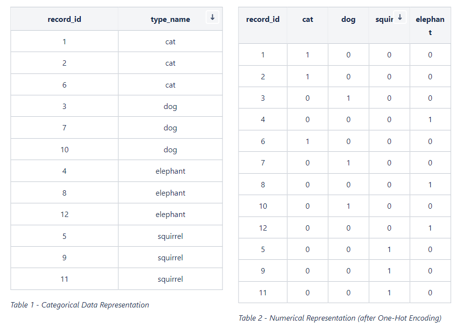
In the datasets that we are currently dealing with, we have a categorical variable as the output (i.e. 43 classes for representing the output). While some algorithms are capable of dealing with categorical data, many of the algorithms are comfortable on dealing with numerical data instead of the categorical data. One-Hot Encoding is a conversion process for representing categorical data numerically. Imagine that we are developing an animal classifier and suppose that we have cat, dog, squirrel, and elephant as the set of types of animals (as shown in Table 1). Once the One-Hot Encoding is applied to the data given in Table 1, the output becomes a numerical representation as depicted in Table 2.
For One-Hot Encoding, we use the function given below.
def convert_to_one_hot(Y, C):
    Y = np.eye(C)[Y.reshape(-1)].T
    return Y
The following code snippet shows how we applied the One-Hot Encoding to data corresponding to the output (Y) from all the available datasets. The code snippet further shows shapes of the numpy arrays after all the previously followed steps.
Y_train = convert_to_one_hot(Y_train_orig, 43).T
Y_val = convert_to_one_hot(Y_val_orig, 43).T
Y_test = convert_to_one_hot(Y_test_orig, 43).T
Y_sv_test = convert_to_one_hot(Y_sv_test_orig, 43).T

print ("Number of Training Examples = " + str(X_train.shape[0]))  // 31367
print ("Number of Validation Examples = " + str(X_val.shape[0]))  // 7842
print ("Number of Test Examples = " + str(X_val.shape[0]))        // 12630
print("X_train shape: " + str(X_train.shape))                     // (31367, 30, 30, 3)
print("Y_train shape: " + str(Y_train.shape))                     // (31367, 43)
print("X_val shape: " + str(X_val.shape))                         // (7842, 30, 30, 3)
print("Y_val shape: " + str(Y_val.shape))                         // (7842, 43)
print("X_test shape: " + str(X_test.shape))                       // (12630, 30, 30, 3)
print("Y_test shape: " + str(Y_test.shape))                       // (12630, 43)
print("X_sv_test shape: " + str(X_sv_test.shape))                 // (32, 30, 30, 3)
print("Y_sv_test shape: " + str(Y_sv_test.shape))                 // (32, 43)
Array to Image
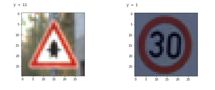
If you are curious, you can always convert an array representation of an image to an image, and see the how it actually looks like. The following code snippets show how you can convert an array back to an image.
Sample image from the Train dataset
# Sample image from the Train dataset # Sample image from Street View Sample
index = 36 index = 24
plt.imshow(X_train[index]) plt.imshow(X_sv_test[index])
print ("y = " + str(np.squeeze(Y_train_orig[index]))) print ("y = " + str(np.squeeze(Y_sv_test_orig[index])))
Setting up Commonly Used Functions
We realized that there are tasks that required us to follow almost the same procedure with slight adjustments to the code. From a programming perspective, this is an area where the usage of functions come in handy. We coded up three functions to encapsulate three tasks: 1) Training and Plotting; 2) Plotting; and 3) Evaluation
The following code snippet displays the code blocks used by us. Feel free to make adjustments wherever necessary.
Common Functions
def train_and_plot(model, epochs = 10, batch_size = 64):
train_dataset = tf.data.Dataset.from_tensor_slices((X_train, Y_train)).batch(batch_size)
val_dataset = tf.data.Dataset.from_tensor_slices((X_val, Y_val)).batch(batch_size )
history = model.fit(train_dataset, epochs = epochs, validation_data=val_dataset)
plot(history)
def plot(history):
# Plotting the Accuracy variation
plt.figure(0)
plt.plot(history.history['accuracy'], label='Training Accuracy')
plt.plot(history.history['val_accuracy'], label='Validation Accuracy')
plt.title('Variation of Accuracy')
plt.xlabel('Epochs')
plt.ylabel('Accuracy')
plt.legend()
plt.show()
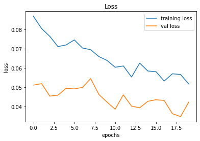
# Plotting the Loss variation
plt.figure(1)
plt.plot(history.history['loss'], label='Training Loss')
plt.plot(history.history['val_loss'], label='Validation Loss')
plt.title('Loss')
plt.xlabel('Epochs')
plt.ylabel('Loss')
plt.legend()
plt.show()
def evaluate_validation(model, no_of_images, rows, columns, dataset_type):
X_ds = None
Y_ds = None
Y_orig_ds = None
result_title = None
if dataset_type == 'test':
X_ds = X_test
Y_ds = Y_test
Y_orig_ds = Y_test_orig
result_title = "TEST"
elif dataset_type == 'val':
X_ds = X_val
Y_ds = Y_val
Y_orig_ds = Y_val_orig
result_title = "VALIDATION"
else:
X_ds = X_sv_test
Y_ds = Y_sv_test
Y_orig_ds = Y_sv_test_orig
result_title = "STREETVIEW TEST"
eval_result = model.evaluate(X_ds, Y_ds)
pred = model.predict(X_ds)
pred_label = [np.argmax(x) for x in pred]
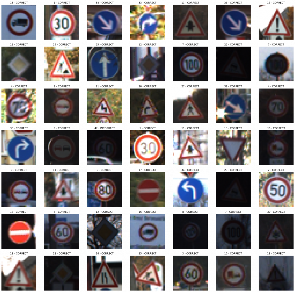
plt.figure(figsize=(25, 25))
for i in range(no_of_images):
plt.subplot(rows, columns, i + 1)
if (pred_label[i] == Y_orig_ds[i]):
plt.title(str(pred_label[i]) + " - CORRECT")
else:
plt.title(str(pred_label[i]) + " - INCORRECT")
plt.imshow(X_ds[i])
plt.axis("off")
plt.show()
y_actu = pd.Series(Y_orig_ds, name='Actual')
y_pred = pd.Series(pred_label, name='Predicted')
conf_matrix = pd.crosstab(y_actu, y_pred)
print(conf_matrix)
accuracy = np.diag(conf_matrix).sum() / conf_matrix.to_numpy().sum()
print("######################")
print(result_title + " Accuracy: " + str(round(eval_result[1],4)*100) + "%")
print("######################")
Model Development - The Iterative Cycle
This will be the longest section of the article as we attempt to explain the thought process behind each tried and tested model. For each model, we will try to be as descriptive as possible and the corresponding results of each model, will also be shown in this section itself (rather than using a different section for Results).
In this section, you will be guided through the process followed by us in implementing and improving the models in an iterative manner. Since this is an iterative procedure, the model accuracy was considered as the single number evaluation metric, and the improvements/modifications are made to models based on the result of the model accuracy obtained by evaluating the validation dataset.
Model 001
The initial model was created to represent the most basic neural network with Input > Dense where we used Adam as the optimizer.
def convolutional_model(input_shape):
input_img = tf.keras.Input(shape=input_shape)
F = tf.keras.layers.Flatten()(input_img)
outputs = tf.keras.layers.Dense(units = 43, activation = 'softmax')(F)
model = tf.keras.Model(inputs=input_img, outputs=outputs)
return model
conv_model_v1 = convolutional_model((30, 30, 3))
conv_model_v1.compile(optimizer='adam',
loss='categorical_crossentropy',
metrics=['accuracy'])
conv_model_v1.summary()
train_and_plot(conv_model_v1)
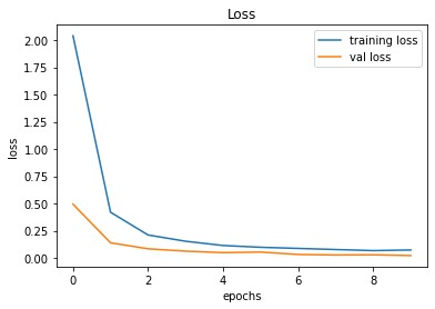
evaluate_validation(model = conv_model_v1, no_of_images = 32, rows = 7, columns = 7, type = 'val')Upon training and plotting, the following outcome was obtained. As it turned out, a validation accuracy of 90.16% was achieved. For a basic neural network, this was an excellent result.
Training and Plotting Results - Model 001

Epoch 1/10
491/491 [==============================] - 2s 4ms/step - loss: 2.0973 - accuracy: 0.5373 - val_loss: 1.4628 - val_accuracy: 0.7042
Epoch 2/10
491/491 [==============================] - 2s 3ms/step - loss: 1.2372 - accuracy: 0.7553 - val_loss: 1.0785 - val_accuracy: 0.7844
Epoch 3/10
491/491 [==============================] - 2s 3ms/step - loss: 0.9560 - accuracy: 0.8221 - val_loss: 0.8889 - val_accuracy: 0.8213
Epoch 4/10
491/491 [==============================] - 2s 3ms/step - loss: 0.7964 - accuracy: 0.8552 - val_loss: 0.7673 - val_accuracy: 0.8475
Epoch 5/10
491/491 [==============================] - 2s 3ms/step - loss: 0.6903 - accuracy: 0.8755 - val_loss: 0.6821 - val_accuracy: 0.8671
Epoch 6/10
491/491 [==============================] - 2s 3ms/step - loss: 0.6133 - accuracy: 0.8893 - val_loss: 0.6203 - val_accuracy: 0.8795
Epoch 7/10
491/491 [==============================] - 2s 3ms/step - loss: 0.5540 - accuracy: 0.8992 - val_loss: 0.5724 - val_accuracy: 0.8898
Epoch 8/10
491/491 [==============================] - 2s 3ms/step - loss: 0.5067 - accuracy: 0.9078 - val_loss: 0.5360 - val_accuracy: 0.8949
Epoch 9/10
491/491 [==============================] - 2s 3ms/step - loss: 0.4680 - accuracy: 0.9141 - val_loss: 0.5084 - val_accuracy: 0.8999
Epoch 10/10
491/491 [==============================] - 2s 3ms/step - loss: 0.4354 - accuracy: 0.9195 - val_loss: 0.4859 - val_accuracy: 0.9016
246/246 [==============================] - 0s 2ms/step - loss: 0.4859 - accuracy: 0.9016
######################
VALIDATION Accuracy: 90.16%
######################
Model 002
In this model, the Model 001 is improved by adding a convolutional layer.
def convolutional_model(input_shape):
input_img = tf.keras.Input(shape=input_shape)
Z1 = tf.keras.layers.Conv2D(filters=32, kernel_size= (5, 5), activation = 'relu')(input_img)
F = tf.keras.layers.Flatten()(Z1)
outputs = tf.keras.layers.Dense(units = 43, activation = 'softmax')(F)
model = tf.keras.Model(inputs=input_img, outputs=outputs)
return model
conv_model_v2 = convolutional_model((30, 30, 3))
conv_model_v2.compile(optimizer='adam',
loss='categorical_crossentropy',
metrics=['accuracy'])
conv_model_v2.summary()
train_and_plot(conv_model_v2, epochs = 10)
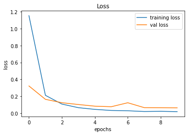
evaluate_validation(model = conv_model_v2, no_of_images = 49, rows = 7, columns = 7, type = 'val')After training, the validation accuracy was increased by the model up to 97.13%. Can we improve it further?
Validation Accuracy of Model 001 = 90.16%Validation Accuracy of Model 002 = 97.13%
Training and Plotting Results - Model 002

Epoch 1/10
491/491 [==============================] - 14s 29ms/step - loss: 0.8728 - accuracy: 0.7880 - val_loss: 0.3256 - val_accuracy: 0.9299
Epoch 2/10
491/491 [==============================] - 14s 29ms/step - loss: 0.2117 - accuracy: 0.9495 - val_loss: 0.2012 - val_accuracy: 0.9569
Epoch 3/10
491/491 [==============================] - 14s 28ms/step - loss: 0.1183 - accuracy: 0.9723 - val_loss: 0.1655 - val_accuracy: 0.9647
Epoch 4/10
491/491 [==============================] - 14s 29ms/step - loss: 0.0850 - accuracy: 0.9796 - val_loss: 0.1794 - val_accuracy: 0.9588
Epoch 5/10
491/491 [==============================] - 14s 29ms/step - loss: 0.0725 - accuracy: 0.9821 - val_loss: 0.1592 - val_accuracy: 0.9663
Epoch 6/10
491/491 [==============================] - 14s 29ms/step - loss: 0.0491 - accuracy: 0.9869 - val_loss: 0.1543 - val_accuracy: 0.9644
Epoch 7/10
491/491 [==============================] - 15s 30ms/step - loss: 0.0519 - accuracy: 0.9866 - val_loss: 0.1247 - val_accuracy: 0.9748
Epoch 8/10
491/491 [==============================] - 14s 29ms/step - loss: 0.0389 - accuracy: 0.9898 - val_loss: 0.1205 - val_accuracy: 0.9773
Epoch 9/10
491/491 [==============================] - 14s 29ms/step - loss: 0.0301 - accuracy: 0.9928 - val_loss: 0.1227 - val_accuracy: 0.9773
Epoch 10/10
491/491 [==============================] - 15s 30ms/step - loss: 0.0271 - accuracy: 0.9930 - val_loss: 0.1390 - val_accuracy: 0.9713
246/246 [==============================] - 1s 6ms/step - loss: 0.1390 - accuracy: 0.9713
Model 003
This is an attempted improvement from Model 002 by adding a MaxPool2D layer.
def convolutional_model(input_shape):
    input_img = tf.keras.Input(shape=input_shape)
    Z1 = tf.keras.layers.Conv2D(filters=32, kernel_size= (5, 5), activation = 'relu')(input_img)
    P1 = tf.keras.layers.MaxPool2D(pool_size=(2, 2))(Z1)
    F = tf.keras.layers.Flatten()(P1)
    outputs = tf.keras.layers.Dense(units = 43, activation = 'softmax')(F)
    model = tf.keras.Model(inputs=input_img, outputs=outputs)
    return model

conv_model_v3 = convolutional_model((30, 30, 3))
conv_model_v3.compile(optimizer='adam',
                  loss='categorical_crossentropy',
                  metrics=['accuracy'])
conv_model_v3.summary()
train_and_plot(conv_model_v3, epochs = 10)
evaluate_validation(model = conv_model_v3, no_of_images = 49, rows = 7, columns = 7, type = 'val')
The results between Model 002 and Model 003 are similar. However, there's a noticeable difference between the Training Error and Validation Error and this is an indication of overfitting.
Validation Accuracy of Model 002 = 97.13%Validation Accuracy of Model 003 = 97.45%
Training and Plotting Results - Model 003

Epoch 1/10
491/491 [==============================] - 15s 30ms/step - loss: 1.0802 - accuracy: 0.7429 - val_loss: 0.3993 - val_accuracy: 0.9161
Epoch 2/10
491/491 [==============================] - 15s 30ms/step - loss: 0.2667 - accuracy: 0.9440 - val_loss: 0.2223 - val_accuracy: 0.9510
Epoch 3/10
491/491 [==============================] - 15s 31ms/step - loss: 0.1482 - accuracy: 0.9693 - val_loss: 0.1708 - val_accuracy: 0.9610
Epoch 4/10
491/491 [==============================] - 15s 30ms/step - loss: 0.0971 - accuracy: 0.9806 - val_loss: 0.1510 - val_accuracy: 0.9648
Epoch 5/10
491/491 [==============================] - 16s 32ms/step - loss: 0.0702 - accuracy: 0.9862 - val_loss: 0.1266 - val_accuracy: 0.9727
Epoch 6/10
491/491 [==============================] - 15s 32ms/step - loss: 0.0546 - accuracy: 0.9887 - val_loss: 0.1272 - val_accuracy: 0.9709
Epoch 7/10
491/491 [==============================] - 16s 33ms/step - loss: 0.0561 - accuracy: 0.9885 - val_loss: 0.1198 - val_accuracy: 0.9754
Epoch 8/10
491/491 [==============================] - 15s 31ms/step - loss: 0.0422 - accuracy: 0.9911 - val_loss: 0.1137 - val_accuracy: 0.9770
Epoch 9/10
491/491 [==============================] - 15s 31ms/step - loss: 0.0338 - accuracy: 0.9925 - val_loss: 0.1097 - val_accuracy: 0.9762
Epoch 10/10
491/491 [==============================] - 16s 32ms/step - loss: 0.0277 - accuracy: 0.9942 - val_loss: 0.1169 - val_accuracy: 0.9745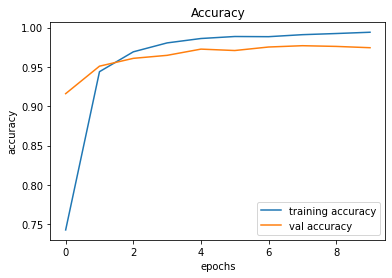
246/246 [==============================] - 1s 6ms/step - loss: 0.1169 - accuracy: 0.9745
Model 004
We will add another Convolutional Layer too see if the results improve to minimize the bias (before focusing on the overfitting problems).
def convolutional_model(input_shape):
    input_img = tf.keras.Input(shape=input_shape)
    Z1 = tf.keras.layers.Conv2D(filters=32, kernel_size= (5, 5), activation = 'relu')(input_img)
    P1 = tf.keras.layers.MaxPool2D(pool_size=(2, 2))(Z1)
    Z2 = tf.keras.layers.Conv2D(filters=64, kernel_size= (5, 5), activation = 'relu')(P1)
    F = tf.keras.layers.Flatten()(Z2)
    outputs = tf.keras.layers.Dense(units = 43, activation = 'softmax')(F)
    model = tf.keras.Model(inputs=input_img, outputs=outputs)
    return model

conv_model_v4 = convolutional_model((30, 30, 3))
conv_model_v4.compile(optimizer='adam',
                  loss='categorical_crossentropy',
                  metrics=['accuracy'])
conv_model_v4.summary()
train_and_plot(conv_model_v4, epochs = 10)
evaluate_validation(model = conv_model_4, no_of_images = 49, rows = 7, columns = 7, type = 'val')
While the validation accuracy improved by approximately 1%, the overfitting problem remains an issue due to the difference between the Training Error and Validation Error.
Validation Accuracy of Model 003 = 97.45%Validation Accuracy of Model 004 = 98.51%
Training and Plotting Results - Model 004

Epoch 1/10
491/491 [==============================] - 26s 53ms/step - loss: 0.8186 - accuracy: 0.7919 - val_loss: 0.2310 - val_accuracy: 0.9498
Epoch 2/10
491/491 [==============================] - 27s 55ms/step - loss: 0.1544 - accuracy: 0.9647 - val_loss: 0.1435 - val_accuracy: 0.9675
Epoch 3/10
491/491 [==============================] - 30s 60ms/step - loss: 0.0759 - accuracy: 0.9824 - val_loss: 0.0957 - val_accuracy: 0.9800
Epoch 4/10
491/491 [==============================] - 29s 59ms/step - loss: 0.0426 - accuracy: 0.9901 - val_loss: 0.0951 - val_accuracy: 0.9796
Epoch 5/10
491/491 [==============================] - 28s 58ms/step - loss: 0.0297 - accuracy: 0.9926 - val_loss: 0.0839 - val_accuracy: 0.9837
Epoch 6/10
491/491 [==============================] - 28s 56ms/step - loss: 0.0223 - accuracy: 0.9942 - val_loss: 0.0870 - val_accuracy: 0.9813
Epoch 7/10
491/491 [==============================] - 27s 55ms/step - loss: 0.0221 - accuracy: 0.9947 - val_loss: 0.0908 - val_accuracy: 0.9816
Epoch 8/10
491/491 [==============================] - 27s 56ms/step - loss: 0.0247 - accuracy: 0.9931 - val_loss: 0.0877 - val_accuracy: 0.9836
Epoch 9/10
491/491 [==============================] - 27s 56ms/step - loss: 0.0110 - accuracy: 0.9973 - val_loss: 0.1071 - val_accuracy: 0.9821
Epoch 10/10
491/491 [==============================] - 28s 57ms/step - loss: 0.0069 - accuracy: 0.9984 - val_loss: 0.0817 - val_accuracy: 0.9851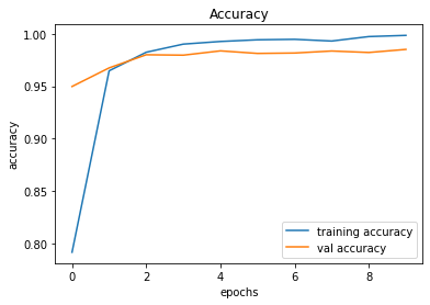
246/246 [==============================] - 2s 8ms/step - loss: 0.0817 - accuracy: 0.9851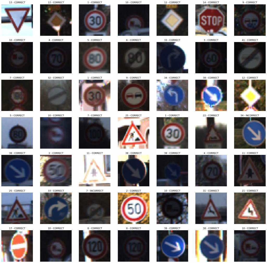
Model 005
We will add another MaxPooling2D Layer before going ahead with the regularization to tackle the overfitting problem.
def convolutional_model(input_shape):
    input_img = tf.keras.Input(shape=input_shape)
    Z1 = tf.keras.layers.Conv2D(filters=32, kernel_size= (5, 5), activation = 'relu')(input_img)
    P1 = tf.keras.layers.MaxPool2D(pool_size=(2, 2))(Z1)
    Z2 = tf.keras.layers.Conv2D(filters=64, kernel_size= (5, 5), activation = 'relu')(P1)
    P2 = tf.keras.layers.MaxPool2D(pool_size=(2, 2))(Z2)
    F = tf.keras.layers.Flatten()(P2)
    outputs = tf.keras.layers.Dense(units = 43, activation = 'softmax')(F)
    model = tf.keras.Model(inputs=input_img, outputs=outputs)
    return model

conv_model_v5 = convolutional_model((30, 30, 3))
conv_model_v5.compile(optimizer='adam',
                  loss='categorical_crossentropy',
                  metrics=['accuracy'])
conv_model_v5.summary()
train_and_plot(conv_model_v8, epochs = 10)
There is a slight improvement in the validation accuracy from 98.51% to 98.83%. However, there is still a slight difference between the training and validation accuracies.
Validation Accuracy of Model 004 = 98.51%Validation Accuracy of Model 005 = 98.83%
Training and Plotting Results - Model 005

Epoch 1/10
491/491 [==============================] - 25s 51ms/step - loss: 1.1546 - accuracy: 0.7134 - val_loss: 0.3212 - val_accuracy: 0.9245
Epoch 2/10
491/491 [==============================] - 25s 50ms/step - loss: 0.2106 - accuracy: 0.9515 - val_loss: 0.1631 - val_accuracy: 0.9611
Epoch 3/10
491/491 [==============================] - 26s 53ms/step - loss: 0.1069 - accuracy: 0.9764 - val_loss: 0.1229 - val_accuracy: 0.9697
Epoch 4/10
491/491 [==============================] - 26s 54ms/step - loss: 0.0641 - accuracy: 0.9858 - val_loss: 0.1016 - val_accuracy: 0.9749
Epoch 5/10
491/491 [==============================] - 27s 54ms/step - loss: 0.0441 - accuracy: 0.9908 - val_loss: 0.0819 - val_accuracy: 0.9815
Epoch 6/10
491/491 [==============================] - 26s 54ms/step - loss: 0.0311 - accuracy: 0.9936 - val_loss: 0.0754 - val_accuracy: 0.9829
Epoch 7/10
491/491 [==============================] - 27s 55ms/step - loss: 0.0274 - accuracy: 0.9935 - val_loss: 0.1225 - val_accuracy: 0.9750
Epoch 8/10
491/491 [==============================] - 26s 53ms/step - loss: 0.0188 - accuracy: 0.9956 - val_loss: 0.0646 - val_accuracy: 0.9846
Epoch 9/10
491/491 [==============================] - 25s 51ms/step - loss: 0.0211 - accuracy: 0.9951 - val_loss: 0.0637 - val_accuracy: 0.9866
Epoch 10/10
491/491 [==============================] - 25s 51ms/step - loss: 0.0170 - accuracy: 0.9960 - val_loss: 0.0621 - val_accuracy: 0.9883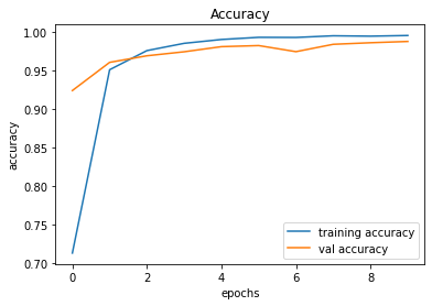
246/246 [==============================] - 2s 8ms/step - loss: 0.0621 - accuracy: 0.9883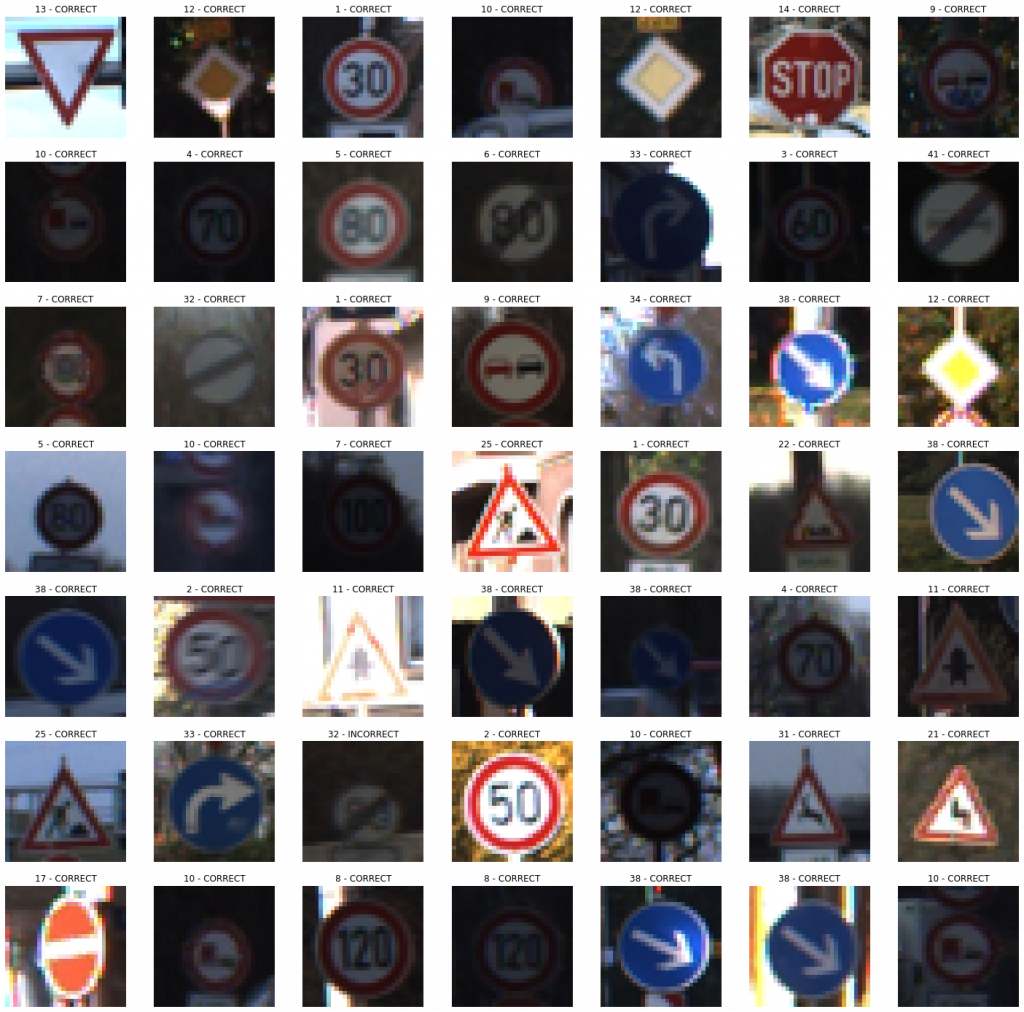
Model 006
Because of the difference between the training and validation accuracies, we are now adding a Dropout layer to address the overfitting problem.
def convolutional_model(input_shape):
input_img = tf.keras.Input(shape=input_shape)
Z1 = tf.keras.layers.Conv2D(filters=32, kernel_size= (5, 5), activation = 'relu')(input_img)
P1 = tf.keras.layers.MaxPool2D(pool_size=(2, 2))(Z1)
D1 = tf.keras.layers.Dropout(rate = 0.25)(P1)
Z2 = tf.keras.layers.Conv2D(filters=64, kernel_size= (5, 5), activation = 'relu')(D1)
P2 = tf.keras.layers.MaxPool2D(pool_size=(2, 2))(Z2)
F = tf.keras.layers.Flatten()(P2)
outputs = tf.keras.layers.Dense(units = 43, activation = 'softmax')(F)
model = tf.keras.Model(inputs=input_img, outputs=outputs)
return model
conv_model_v6 = convolutional_model((30, 30, 3))
conv_model_v6.compile(optimizer='adam',
loss='categorical_crossentropy',
metrics=['accuracy'])
conv_model_v6.summary()
train_and_plot(conv_model_v6, epochs = 10)
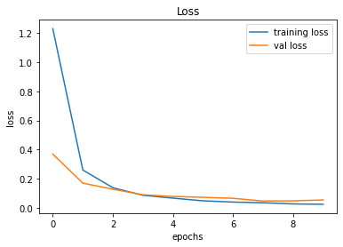
evaluate_validation(model = conv_model_v6, no_of_images = 49, rows = 7, columns = 7, type = 'val')The Dropout certainly had an effect in narrowing down the gap between Training Error and Validation Error. However, there is an indication of validation accuracy going down after Epoch 09. In such cases, Early Stopping may come in handy.
Validation Accuracy of Model 005 = 98.83%Validation Accuracy of Model 006 = 98.83%
Training and Plotting Results - Model 006

Epoch 1/10
491/491 [==============================] - 29s 59ms/step - loss: 1.2292 - accuracy: 0.6867 - val_loss: 0.3695 - val_accuracy: 0.9115
Epoch 2/10
491/491 [==============================] - 29s 59ms/step - loss: 0.2606 - accuracy: 0.9351 - val_loss: 0.1708 - val_accuracy: 0.9634
Epoch 3/10
491/491 [==============================] - 30s 62ms/step - loss: 0.1393 - accuracy: 0.9661 - val_loss: 0.1292 - val_accuracy: 0.9686
Epoch 4/10
491/491 [==============================] - 30s 61ms/step - loss: 0.0874 - accuracy: 0.9791 - val_loss: 0.0912 - val_accuracy: 0.9802
Epoch 5/10
491/491 [==============================] - 29s 59ms/step - loss: 0.0680 - accuracy: 0.9835 - val_loss: 0.0797 - val_accuracy: 0.9815
Epoch 6/10
491/491 [==============================] - 29s 59ms/step - loss: 0.0496 - accuracy: 0.9882 - val_loss: 0.0736 - val_accuracy: 0.9847
Epoch 7/10
491/491 [==============================] - 30s 60ms/step - loss: 0.0411 - accuracy: 0.9896 - val_loss: 0.0669 - val_accuracy: 0.9846
Epoch 8/10
491/491 [==============================] - 29s 60ms/step - loss: 0.0362 - accuracy: 0.9899 - val_loss: 0.0481 - val_accuracy: 0.9894
Epoch 9/10
491/491 [==============================] - 30s 60ms/step - loss: 0.0285 - accuracy: 0.9928 - val_loss: 0.0496 - val_accuracy: 0.9888
Epoch 10/10
491/491 [==============================] - 30s 61ms/step - loss: 0.0259 - accuracy: 0.9936 - val_loss: 0.0557 - val_accuracy: 0.9883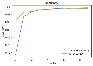
246/246 [==============================] - 2s 8ms/step - loss: 0.0557 - accuracy: 0.9883
Model 007
We will add another Dropout layer to see if we can further fine-tune the model and then let's proceed with Early Stopping if necessary.
# Model 007
def convolutional_model(input_shape):
input_img = tf.keras.Input(shape=input_shape)
Z1 = tf.keras.layers.Conv2D(filters=32, kernel_size= (5, 5), activation = 'relu')(input_img)
P1 = tf.keras.layers.MaxPool2D(pool_size=(2, 2))(Z1)
D1 = tf.keras.layers.Dropout(rate = 0.25)(P1)
Z2 = tf.keras.layers.Conv2D(filters=64, kernel_size= (5, 5), activation = 'relu')(D1)
P2 = tf.keras.layers.MaxPool2D(pool_size=(2, 2))(Z2)
D2 = tf.keras.layers.Dropout(rate = 0.25)(P2)
F = tf.keras.layers.Flatten()(D2)
outputs = tf.keras.layers.Dense(units = 43, activation = 'softmax')(F)
model = tf.keras.Model(inputs=input_img, outputs=outputs)
return model
conv_model_v7 = convolutional_model((30, 30, 3))
conv_model_v7.compile(optimizer='adam',
loss='categorical_crossentropy',
metrics=['accuracy'])
conv_model_v7.summary()
train_and_plot(conv_model_v7, epochs = 10)
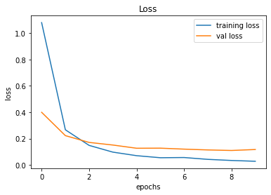
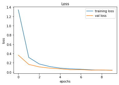
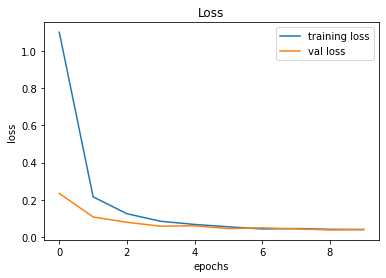
evaluate_validation(model = conv_model_v7, no_of_images = 49, rows = 7, columns = 7, type = 'val')The validation accuracy slightly improved from 98.83% to 99.22%.
Validation Accuracy of Model 006 = 98.83%Validation Accuracy of Model 007 = 99.22%
Training and Plotting Results - Model 007

Epoch 1/10
491/491 [==============================] - 30s 61ms/step - loss: 1.3423 - accuracy: 0.6474 - val_loss: 0.3653 - val_accuracy: 0.9217
Epoch 2/10
491/491 [==============================] - 30s 62ms/step - loss: 0.3166 - accuracy: 0.9155 - val_loss: 0.1653 - val_accuracy: 0.9675
Epoch 3/10
491/491 [==============================] - 31s 64ms/step - loss: 0.1760 - accuracy: 0.9539 - val_loss: 0.1124 - val_accuracy: 0.9784
Epoch 4/10
491/491 [==============================] - 36s 74ms/step - loss: 0.1198 - accuracy: 0.9687 - val_loss: 0.0857 - val_accuracy: 0.9844
Epoch 5/10
491/491 [==============================] - 39s 80ms/step - loss: 0.0861 - accuracy: 0.9769 - val_loss: 0.0709 - val_accuracy: 0.9837
Epoch 6/10
491/491 [==============================] - 32s 66ms/step - loss: 0.0710 - accuracy: 0.9808 - val_loss: 0.0517 - val_accuracy: 0.9892
Epoch 7/10
491/491 [==============================] - 41s 84ms/step - loss: 0.0621 - accuracy: 0.9830 - val_loss: 0.0535 - val_accuracy: 0.9895
Epoch 8/10
491/491 [==============================] - 34s 68ms/step - loss: 0.0486 - accuracy: 0.9868 - val_loss: 0.0422 - val_accuracy: 0.9922
Epoch 9/10
491/491 [==============================] - 30s 61ms/step - loss: 0.0424 - accuracy: 0.9881 - val_loss: 0.0458 - val_accuracy: 0.9903
Epoch 10/10
491/491 [==============================] - 30s 62ms/step - loss: 0.0416 - accuracy: 0.9881 - val_loss: 0.0387 - val_accuracy: 0.9922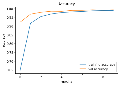
246/246 [==============================] - 2s 8ms/step - loss: 0.0387 - accuracy: 0.9922
Model 008
Adding more layers make the network deeper and having a bigger network almost always helps in minimizing the bias, and for increasing the accuracy. Therefore, we will add another Convolutional Layer to see if we can further increase the Validation Accuracy. On the other hand, the validation accuracy surpassed the training accuracy, and this happens due to the effect of Dropout.
def convolutional_model(input_shape):
input_img = tf.keras.Input(shape=input_shape)
Z1 = tf.keras.layers.Conv2D(filters=32, kernel_size= (5, 5), activation = 'relu')(input_img)
P1 = tf.keras.layers.MaxPool2D(pool_size=(2, 2))(Z1)
D1 = tf.keras.layers.Dropout(rate = 0.25)(P1)
Z2 = tf.keras.layers.Conv2D(filters=64, kernel_size= (5, 5), activation = 'relu')(D1)
P2 = tf.keras.layers.MaxPool2D(pool_size=(2, 2))(Z2)
D2 = tf.keras.layers.Dropout(rate = 0.25)(P2)
Z3 = tf.keras.layers.Conv2D(filters=256, kernel_size= (3, 3), activation = 'relu')(D2)
F = tf.keras.layers.Flatten()(Z3)
outputs = tf.keras.layers.Dense(units = 43, activation = 'softmax')(F)
model = tf.keras.Model(inputs=input_img, outputs=outputs)
return model
conv_model_v8 = convolutional_model((30, 30, 3))
conv_model_v8.compile(optimizer='adam',
loss='categorical_crossentropy',
metrics=['accuracy'])
conv_model_v8.summary()
train_and_plot(conv_model_v8, epochs = 10)
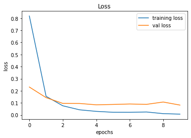
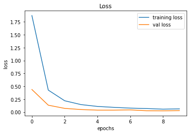
evaluate_validation(model = conv_model_v8, no_of_images = 49, rows = 7, columns = 7, type = 'val')The validation accuracy slightly improved from 99.22% to 99.34%.
Validation Accuracy of Model 007 = 98.22%Validation Accuracy of Model 008 = 99.34%
Training and Plotting Results - Model 008
Epoch 1/10
491/491 [==============================] - 31s 63ms/step - loss: 1.1019 - accuracy: 0.6988 - val_loss: 0.2339 - val_accuracy: 0.9439
Epoch 2/10
491/491 [==============================] - 32s 65ms/step - loss: 0.2157 - accuracy: 0.9404 - val_loss: 0.1071 - val_accuracy: 0.9740
Epoch 3/10
491/491 [==============================] - 35s 72ms/step - loss: 0.1245 - accuracy: 0.9656 - val_loss: 0.0783 - val_accuracy: 0.9830
Epoch 4/10
491/491 [==============================] - 33s 67ms/step - loss: 0.0837 - accuracy: 0.9761 - val_loss: 0.0574 - val_accuracy: 0.9892
Epoch 5/10
491/491 [==============================] - 34s 70ms/step - loss: 0.0669 - accuracy: 0.9806 - val_loss: 0.0595 - val_accuracy: 0.9884
Epoch 6/10
491/491 [==============================] - 33s 68ms/step - loss: 0.0540 - accuracy: 0.9848 - val_loss: 0.0446 - val_accuracy: 0.9926
Epoch 7/10
491/491 [==============================] - 35s 71ms/step - loss: 0.0424 - accuracy: 0.9877 - val_loss: 0.0486 - val_accuracy: 0.9899
Epoch 8/10
491/491 [==============================] - 33s 68ms/step - loss: 0.0447 - accuracy: 0.9868 - val_loss: 0.0429 - val_accuracy: 0.9911
Epoch 9/10
491/491 [==============================] - 36s 73ms/step - loss: 0.0405 - accuracy: 0.9879 - val_loss: 0.0373 - val_accuracy: 0.9930
Epoch 10/10
491/491 [==============================] - 38s 78ms/step - loss: 0.0393 - accuracy: 0.9881 - val_loss: 0.0392 - val_accuracy: 0.9934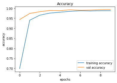
246/246 [==============================] - 2s 10ms/step - loss: 0.0392 - accuracy: 0.9934
Model 009
We further add another MaxPool2D layer, followed by a Dropout layer.
def convolutional_model(input_shape):
    input_img = tf.keras.Input(shape=input_shape)
    Z1 = tf.keras.layers.Conv2D(filters=32, kernel_size= (5, 5), activation = 'relu')(input_img)
    P1 = tf.keras.layers.MaxPool2D(pool_size=(2, 2))(Z1)
    D1 = tf.keras.layers.Dropout(rate = 0.25)(P1)
    Z2 = tf.keras.layers.Conv2D(filters=64, kernel_size= (5, 5), activation = 'relu')(D1)
    P2 = tf.keras.layers.MaxPool2D(pool_size=(2, 2))(Z2)
    D2 = tf.keras.layers.Dropout(rate = 0.25)(P2)
    Z3 = tf.keras.layers.Conv2D(filters=256, kernel_size= (3, 3), activation = 'relu')(D2)
    P3 = tf.keras.layers.MaxPool2D(pool_size=(2, 2))(Z3)
    D3 = tf.keras.layers.Dropout(rate = 0.25)(P3)
    F = tf.keras.layers.Flatten()(D3)
    outputs = tf.keras.layers.Dense(units = 43, activation = 'softmax')(F)
    model = tf.keras.Model(inputs=input_img, outputs=outputs)
    return model

conv_model_v9 = convolutional_model((30, 30, 3))
conv_model_v9.compile(optimizer='adam',
                  loss='categorical_crossentropy',
                  metrics=['accuracy'])
conv_model_v9.summary()
train_and_plot(conv_model_v9, epochs = 10)
evaluate_validation(model = conv_model_v9, no_of_images = 49, rows = 7, columns = 7, type = 'val')
The validation accuracy slightly improved from 99.34% to 99.36%.
Validation Accuracy of Model 008 = 98.34%Validation Accuracy of Model 009 = 99.36%Training and Plotting Result - Model 009
Training and Plotting Results - Model 009

Epoch 1/10
491/491 [==============================] - 32s 64ms/step - loss: 1.8729 - accuracy: 0.4747 - val_loss: 0.4384 - val_accuracy: 0.8979
Epoch 2/10
491/491 [==============================] - 33s 66ms/step - loss: 0.4269 - accuracy: 0.8749 - val_loss: 0.1343 - val_accuracy: 0.9718
Epoch 3/10
491/491 [==============================] - 34s 69ms/step - loss: 0.2201 - accuracy: 0.9376 - val_loss: 0.0722 - val_accuracy: 0.9852
Epoch 4/10
491/491 [==============================] - 34s 69ms/step - loss: 0.1456 - accuracy: 0.9567 - val_loss: 0.0498 - val_accuracy: 0.9895
Epoch 5/10
491/491 [==============================] - 34s 69ms/step - loss: 0.1102 - accuracy: 0.9676 - val_loss: 0.0382 - val_accuracy: 0.9926
Epoch 6/10
491/491 [==============================] - 34s 70ms/step - loss: 0.0923 - accuracy: 0.9729 - val_loss: 0.0380 - val_accuracy: 0.9932
Epoch 7/10
491/491 [==============================] - 34s 69ms/step - loss: 0.0773 - accuracy: 0.9774 - val_loss: 0.0426 - val_accuracy: 0.9902
Epoch 8/10
491/491 [==============================] - 33s 67ms/step - loss: 0.0692 - accuracy: 0.9800 - val_loss: 0.0265 - val_accuracy: 0.9943
Epoch 9/10
491/491 [==============================] - 32s 66ms/step - loss: 0.0570 - accuracy: 0.9839 - val_loss: 0.0249 - val_accuracy: 0.9939
Epoch 10/10
491/491 [==============================] - 32s 65ms/step - loss: 0.0630 - accuracy: 0.9807 - val_loss: 0.0290 - val_accuracy: 0.9936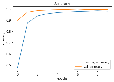
Model 010
Now, we will add a Fully Connected Layer to see if it improves the overall performance (and minimize the bias).
def convolutional_model(input_shape):
    input_img = tf.keras.Input(shape=input_shape)
    Z1 = tf.keras.layers.Conv2D(filters=32, kernel_size= (5, 5), activation = 'relu')(input_img)
    P1 = tf.keras.layers.MaxPool2D(pool_size=(2, 2))(Z1)
    D1 = tf.keras.layers.Dropout(rate = 0.25)(P1)
    Z2 = tf.keras.layers.Conv2D(filters=64, kernel_size= (5, 5), activation = 'relu')(D1)
    P2 = tf.keras.layers.MaxPool2D(pool_size=(2, 2))(Z2)
    D2 = tf.keras.layers.Dropout(rate = 0.25)(P2)
    Z3 = tf.keras.layers.Conv2D(filters=256, kernel_size= (3, 3), activation = 'relu')(D2)
    P3 = tf.keras.layers.MaxPool2D(pool_size=(2, 2))(Z3)
    D3 = tf.keras.layers.Dropout(rate = 0.25)(P3)
    F = tf.keras.layers.Flatten()(D3)
    FC1 = tf.keras.layers.Dense(units = 256, activation = 'relu')(F)
    outputs = tf.keras.layers.Dense(units = 43, activation = 'softmax')(FC1)
    model = tf.keras.Model(inputs=input_img, outputs=outputs)
    return model

conv_model_v10 = convolutional_model((30, 30, 3))
conv_model_v10.compile(optimizer='adam',
                  loss='categorical_crossentropy',
                  metrics=['accuracy'])
conv_model_v10.summary()
train_and_plot(conv_model_v10, epochs = 10)
Validation Accuracy of Model 009 = 98.36%Validation Accuracy of Model 010 = 99.38%
Training and Plotting Results - Model 010

Epoch 1/10
491/491 [==============================] - 31s 63ms/step - loss: 2.0385 - accuracy: 0.4115 - val_loss: 0.4938 - val_accuracy: 0.8601
Epoch 2/10
491/491 [==============================] - 31s 63ms/step - loss: 0.4200 - accuracy: 0.8677 - val_loss: 0.1395 - val_accuracy: 0.9675
Epoch 3/10
491/491 [==============================] - 32s 66ms/step - loss: 0.2112 - accuracy: 0.9377 - val_loss: 0.0846 - val_accuracy: 0.9793
Epoch 4/10
491/491 [==============================] - 32s 65ms/step - loss: 0.1538 - accuracy: 0.9545 - val_loss: 0.0630 - val_accuracy: 0.9856
Epoch 5/10
491/491 [==============================] - 32s 65ms/step - loss: 0.1147 - accuracy: 0.9645 - val_loss: 0.0494 - val_accuracy: 0.9878
Epoch 6/10
491/491 [==============================] - 32s 65ms/step - loss: 0.0984 - accuracy: 0.9698 - val_loss: 0.0545 - val_accuracy: 0.9858
Epoch 7/10
491/491 [==============================] - 32s 66ms/step - loss: 0.0881 - accuracy: 0.9729 - val_loss: 0.0326 - val_accuracy: 0.9918
Epoch 8/10
491/491 [==============================] - 32s 65ms/step - loss: 0.0778 - accuracy: 0.9764 - val_loss: 0.0275 - val_accuracy: 0.9935
Epoch 9/10
491/491 [==============================] - 32s 65ms/step - loss: 0.0679 - accuracy: 0.9787 - val_loss: 0.0291 - val_accuracy: 0.9920
Epoch 10/10
491/491 [==============================] - 32s 66ms/step - loss: 0.0736 - accuracy: 0.9782 - val_loss: 0.0226 - val_accuracy: 0.9938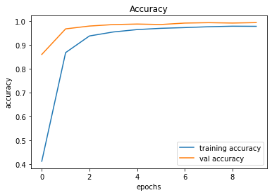
246/246 [==============================] - 2s 9ms/step - loss: 0.0226 - accuracy: 0.9938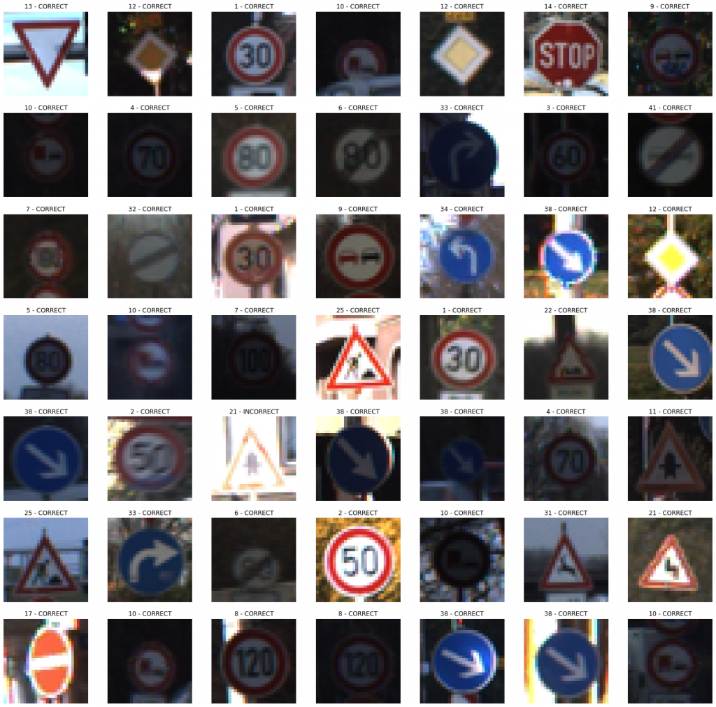
Model 011
While it may not have a considerable effect, it is worth a try to add a regularizer to the Fully Connected Layer.
def convolutional_model(input_shape):
    input_img = tf.keras.Input(shape=input_shape)
    Z1 = tf.keras.layers.Conv2D(filters=32, kernel_size= (5, 5), activation = 'relu')(input_img)
    P1 = tf.keras.layers.MaxPool2D(pool_size=(2, 2))(Z1)
    D1 = tf.keras.layers.Dropout(rate = 0.25)(P1)
    Z2 = tf.keras.layers.Conv2D(filters=64, kernel_size= (5, 5), activation = 'relu')(D1)
    P2 = tf.keras.layers.MaxPool2D(pool_size=(2, 2))(Z2)
    D2 = tf.keras.layers.Dropout(rate = 0.25)(P2)
    Z3 = tf.keras.layers.Conv2D(filters=256, kernel_size= (3, 3), activation = 'relu')(D2)
    P3 = tf.keras.layers.MaxPool2D(pool_size=(2, 2))(Z3)
    D3 = tf.keras.layers.Dropout(rate = 0.25)(P3)
    F = tf.keras.layers.Flatten()(D3)
    FC1 = tf.keras.layers.Dense(units = 256, activation = 'relu', kernel_regularizer=regularizers.l2(0.0001))(F)
    outputs = tf.keras.layers.Dense(units = 43, activation = 'softmax')(FC1)
    model = tf.keras.Model(inputs=input_img, outputs=outputs)
    return model

conv_model_v11 = convolutional_model((30, 30, 3))
conv_model_v11.compile(optimizer='adam',
                  loss='categorical_crossentropy',
                  metrics=['accuracy'])
conv_model_v11.summary()
train_and_plot(conv_model_v11, epochs = 10)
evaluate_validation(model = conv_model_v11, no_of_images = 49, rows = 7, columns = 7, type = 'val')
Validation Accuracy of Model 010 = 99.38%Validation Accuracy of Model 011 = 99.44%
Epoch 1/10
491/491 [==============================] - 32s 66ms/step - loss: 1.9605 - accuracy: 0.4357 - val_loss: 0.5152 - val_accuracy: 0.8624
Epoch 2/10
491/491 [==============================] - 34s 69ms/step - loss: 0.4549 - accuracy: 0.8630 - val_loss: 0.1577 - val_accuracy: 0.9679
Epoch 3/10
491/491 [==============================] - 33s 67ms/step - loss: 0.2494 - accuracy: 0.9301 - val_loss: 0.1195 - val_accuracy: 0.9779
Epoch 4/10
491/491 [==============================] - 32s 66ms/step - loss: 0.1742 - accuracy: 0.9527 - val_loss: 0.0850 - val_accuracy: 0.9860
Epoch 5/10
491/491 [==============================] - 32s 66ms/step - loss: 0.1446 - accuracy: 0.9633 - val_loss: 0.0758 - val_accuracy: 0.9889
Epoch 6/10
491/491 [==============================] - 33s 66ms/step - loss: 0.1236 - accuracy: 0.9696 - val_loss: 0.0676 - val_accuracy: 0.9908
Epoch 7/10
491/491 [==============================] - 33s 67ms/step - loss: 0.1121 - accuracy: 0.9726 - val_loss: 0.0618 - val_accuracy: 0.9918
Epoch 8/10
491/491 [==============================] - 34s 68ms/step - loss: 0.1026 - accuracy: 0.9765 - val_loss: 0.0585 - val_accuracy: 0.9920
Epoch 9/10
491/491 [==============================] - 32s 66ms/step - loss: 0.0965 - accuracy: 0.9778 - val_loss: 0.0539 - val_accuracy: 0.9926
Epoch 10/10
491/491 [==============================] - 33s 66ms/step - loss: 0.0914 - accuracy: 0.9789 - val_loss: 0.0495 - val_accuracy: 0.9944
246/246 [==============================] - 2s 10ms/step - loss: 0.0495 - accuracy: 0.9944
Since we have achieved an acceptable accuracy, let us try to train longer by increasing the number of epochs. While training longer does not always help, it never hurts to try training longer.
train_and_plot(conv_model_v11, epochs = 20)Validation Accuracy of Model 011 (with 10 epochs) = 99.44%Validation Accuracy of Model 011 (with 20 epochs) = 99.53%
Epoch 1/20
491/491 [==============================] - 30s 62ms/step - loss: 0.0867 - accuracy: 0.9806 - val_loss: 0.0511 - val_accuracy: 0.9939
Epoch 2/20
491/491 [==============================] - 32s 64ms/step - loss: 0.0804 - accuracy: 0.9834 - val_loss: 0.0518 - val_accuracy: 0.9938
Epoch 3/20
491/491 [==============================] - 34s 69ms/step - loss: 0.0764 - accuracy: 0.9835 - val_loss: 0.0454 - val_accuracy: 0.9948
Epoch 4/20
491/491 [==============================] - 32s 65ms/step - loss: 0.0710 - accuracy: 0.9849 - val_loss: 0.0459 - val_accuracy: 0.9943
Epoch 5/20
491/491 [==============================] - 31s 64ms/step - loss: 0.0719 - accuracy: 0.9844 - val_loss: 0.0494 - val_accuracy: 0.9927
Epoch 6/20
491/491 [==============================] - 31s 64ms/step - loss: 0.0745 - accuracy: 0.9837 - val_loss: 0.0491 - val_accuracy: 0.9941
Epoch 7/20
491/491 [==============================] - 32s 65ms/step - loss: 0.0703 - accuracy: 0.9855 - val_loss: 0.0499 - val_accuracy: 0.9939
Epoch 8/20
491/491 [==============================] - 32s 65ms/step - loss: 0.0694 - accuracy: 0.9853 - val_loss: 0.0545 - val_accuracy: 0.9926
Epoch 9/20
491/491 [==============================] - 33s 67ms/step - loss: 0.0659 - accuracy: 0.9865 - val_loss: 0.0463 - val_accuracy: 0.9952
Epoch 10/20
491/491 [==============================] - 33s 67ms/step - loss: 0.0639 - accuracy: 0.9875 - val_loss: 0.0423 - val_accuracy: 0.9952
Epoch 11/20
491/491 [==============================] - 36s 72ms/step - loss: 0.0603 - accuracy: 0.9873 - val_loss: 0.0386 - val_accuracy: 0.9954
Epoch 12/20
491/491 [==============================] - 32s 66ms/step - loss: 0.0610 - accuracy: 0.9871 - val_loss: 0.0460 - val_accuracy: 0.9935
Epoch 13/20
491/491 [==============================] - 30s 61ms/step - loss: 0.0553 - accuracy: 0.9898 - val_loss: 0.0402 - val_accuracy: 0.9963
Epoch 14/20
491/491 [==============================] - 34s 69ms/step - loss: 0.0625 - accuracy: 0.9869 - val_loss: 0.0393 - val_accuracy: 0.9960
Epoch 15/20
491/491 [==============================] - 40s 81ms/step - loss: 0.0584 - accuracy: 0.9877 - val_loss: 0.0427 - val_accuracy: 0.9957
Epoch 16/20
491/491 [==============================] - 42s 86ms/step - loss: 0.0580 - accuracy: 0.9881 - val_loss: 0.0435 - val_accuracy: 0.9955
Epoch 17/20
491/491 [==============================] - 37s 76ms/step - loss: 0.0532 - accuracy: 0.9900 - val_loss: 0.0431 - val_accuracy: 0.9952
Epoch 18/20
491/491 [==============================] - 35s 71ms/step - loss: 0.0570 - accuracy: 0.9889 - val_loss: 0.0363 - val_accuracy: 0.9959
Epoch 19/20
491/491 [==============================] - 34s 69ms/step - loss: 0.0566 - accuracy: 0.9889 - val_loss: 0.0348 - val_accuracy: 0.9969
Epoch 20/20
491/491 [==============================] - 34s 70ms/step - loss: 0.0517 - accuracy: 0.9896 - val_loss: 0.0423 - val_accuracy: 0.9953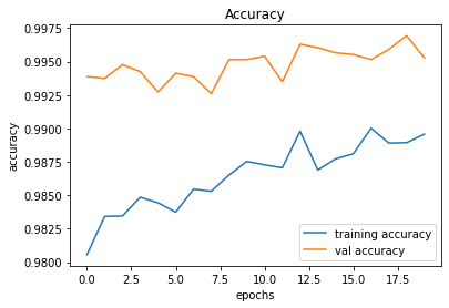
246/246 [==============================] - 2s 8ms/step - loss: 0.0423 - accuracy: 0.9953
We will consider this as the final model because we have been able to achieve a validation accuracy of over 99.50%. The following code snippet should assist us in saving the final model in Hierarchical Data Format version 5 (HDF5).
conv_model_v11.save("gtsrb_v11.h5")Summary
The table given below, summarizes the results of the models that we implemented.
The Test Drive
| Model | Accuracy |
| Model 001 | 90.16% |
| Model 002 | 97.13% |
| Model 003 | 97.45% |
| Model 004 | 98.51% |
| Model 005 | 98.83% |
| Model 006 | 98.83% |
| Model 007 | 99.22% |
| Model 008 | 99.34% |
| Model 009 | 99.36% |
| Model 010 | 99.38% |
| Model 011 | 99.53% |
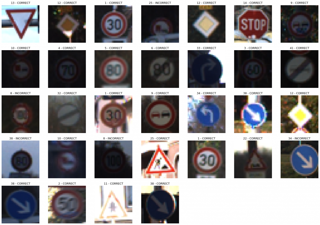
This section is used for explaining the results and implications from the Test phase. The emphasis will be placed for detailing out the specific outcomes from both the Test Dataset and the Custom Street View Test Dataset.
In the previous section, we finally chose Model 011 as the final model because of its high validation accuracy. In this section, we will be applying Model 011 on two completely unseen (left out) Test datasets to see its robustness on a production run. Therefore, the model will be applied first to the Test dataset that came from the original dataset.
evaluate_validation(model = conv_model_v11, no_of_images = 49, rows = 7, columns = 7, type = 'test')395/395 [==============================] - 3s 9ms/step - loss: 0.2013 - accuracy: 0.96371
######################
TEST Accuracy: 96.37%
######################
Voila! The model managed to achieve an accuracy of 96.37% on the completely unseen dataset. Let us see how it performs on the images captured from Google Street View.
evaluate_validation(model = conv_model_v11, no_of_images = 32, rows = 6, columns = 6, type = 'sv')1/1 [==============================] - 0s 1ms/step - loss: 0.0781 - accuracy: 0.9688
######################
STREETVIEW TEST Accuracy: 96.88%
######################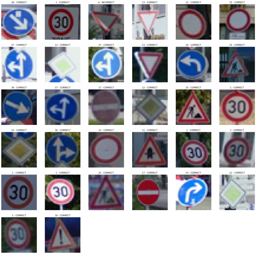
Again, it showed a similar accuracy for a completely unseen dataset. With a little bit of tweaking and troubleshooting, we should be able to improve the performances. But, let us focus on the enhancements on another day. For the moment, we are happy with the output produced by our model.
Do It Yourself!
Here, we will briefly explain how we build a simple, yet effective web application for testing the algorithm on the go. I think that the development of a web app might be beneficial because it showcases our capability to provide an end-to-end solution since we focus on the deployment process as well.
In the previous sections, we demonstrated how you can build a deep learning models from scratch, and test them against different datasets to measure the respective performances. However, we used the Jupyter Notebook interface to handle our coding experiments. We understand the difficulties posed by such an approach if you are a less tech-savvy person. Thus, we hereby present you a handy web application, where the trained models can be utilized by YOURSELF to experience how the models output results.
The application can be reached by visiting the following link, where the necessary instructions have been given for you to easily classify the traffic signs, YOURSELF! Enjoy!
Traffic Sign Recognizer | Do It Yourself!
Feature Additions
Detection of Unknown Images (From 12-07-2021 to 16-07-2021)
After the development of the web application, we realized that the application does not perform up to the expectations when it is presented with an image which does not consist of a trained traffic sign. Since the model had been instructed to strictly output only the designated traffic signs (43), the model was supposed to say that the submitted image belonged to the category of one of the trained traffic signs. This was a problem that we needed to address, and we followed a methodical approach to minimize the issues arising from our problematic approach.
Novelty/Anomaly detection is a research area, where different approaches have been suggested in the literature by the scholars to tackle the problem which we identified. One of the suggested approaches is to include an additional class to the existing list of classes by retraining the model with random images (non-traffic-sign images). Additionally, it is also suggested to create a binary model as a pre-filter which can classify the images by specifying whether the image is a traffic sign or not. For this approach as well, a set of random images are required for training purposes. If we are to follow a different approach, the option is to train a model using an object detection algorithm such as YOLO, and enhance the usability of the web application.
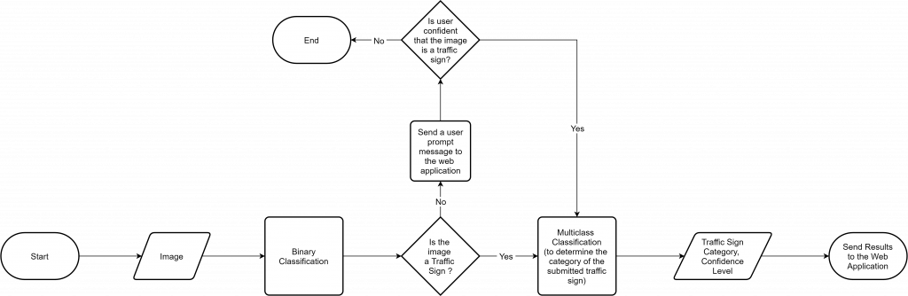
After considering the advantages and disadvantages of the different approaches mentioned above, it was decided to consider one of the first two approaches, because of the comparatively less effort needed to modify our existing model, while meeting our requirement. However, instead of singling out a particular approach, our intention was to implement a solution utilizing both approaches to increase eventual the user experience. As a result, a pre-filter was developed to create a binary classifier which essentially classifies whether an image is a traffic sign or not. After the binary classification, the images are sent through the usual multi-class classifier where the classifier contains an additional class called “Unknown Traffic Sign” to denote images which do not adhere to the characteristics of a trained traffic sign. The following figure illustrates the proposed combined approach.
In order to implement the workflow given in the above figure, the following changes were applied.
Adding “Unknown Traffic Sign” to the existing model
- This process increased the number of classes from 43 to 44.
- To achieve this task, 1930 more random images were added from the COCO Dataset to our training distribution, and assigned the new class label (44: Unknown Traffic Sign) accordingly.
- At the same time, 615 images from the COCO Dataset, were added to the Test dataset.
- The same NN architecture that we had used earlier, was utilized with an additional output class, and the model was retrained to achieve a classification accuracy of 99.57% for the validation dataset.
- The model performed well by minimizing the issues that existed with the recognition of non-traffic-signs.
Development of a binary classifier as a pre-filter
- This process entails the development of a binary classifier which classifies whether an image is a traffic sign or not.
- For this purpose, all the images from the GTSRB Traffic Sign dataset (51,839 images) were considered along with 45,670 images from the COCO dataset (non-traffic-signs).
- Necessary splits and preprocessing tasks were applied before the training process.
- Improved the model iteratively (as we had done in the previous version) to create the binary classifier.
- Managed to achieve a validation accuracy of 99.81% and an accuracy of 99.72% for the left-out Test dataset.
Integration
- As elaborated in the above figure, a submitted image first goes through the binary classifier to detect whether the image is a traffic sign or not. If it is detected as a valid traffic sign, the image will be checked by the traffic sign classifier, and a suitable feedback is sent back to the frontend.
- If the submitted image is detected as a non-traffic-sign image, the user is prompted with a message, and the user confirmation is required to proceed further (to force the application to classify the image regardless of its type).
- If the user wishes to proceed, the image is sent